4 Introduction to Probability

Status: ported 2026-05-19. Reviewed by editor: pending.

Learning outcomes

By the end of this chapter the reader should be able to:

Define a random experiment, sample space, and event, and represent events as subsets of $\Omega$.
Combine events using the standard set operations (union, intersection, complement, difference) and apply De Morgan’s laws.
State Kolmogorov’s three axioms and derive the complement rule, monotonicity, and the inclusion-exclusion formula.
Compute classical (Laplace) probabilities by counting equally likely outcomes.
Compute conditional probabilities $P(A \mid B)$ and apply the multiplication rule, including in tree-diagram problems.
Apply the law of total probability and Bayes’ theorem to update beliefs from prior to posterior given evidence.
Distinguish independence from mutual exclusivity, and recognise common pitfalls (e.g. the base-rate fallacy).
Simulate dice, coins, the birthday paradox, a medical test, and the Monty Hall problem in R.

Motivating empirical question

A rapid test for a disease that affects 1% of the population is 99% sensitive and 95% specific. You test positive. What is the probability that you are actually sick?

The intuitive answer “about 99%” is wrong by an order of magnitude — the correct answer is about 17%. Probability theory, and in particular Bayes’ theorem, is the machinery that turns prior beliefs (the prevalence) and conditional evidence (the test result) into a posterior probability. The same logic governs credit-default models, fraud detection, recession indicators, and insurance pricing. This chapter builds that machinery from the ground up, starting with sample spaces and ending with the false-positive paradox and the Monty Hall problem.

4.1 3.1 Random experiments and sample spaces

In the first two chapters we described data that had already been collected. We now shift to modelling uncertainty: how should we reason about outcomes that have not yet occurred? The mathematical framework is probability theory.

Definition: random experiment

A random experiment (or aleatory experiment) is any process satisfying three conditions:

All possible outcomes can be specified before the experiment is performed.
The actual outcome cannot be predicted with certainty in advance.
The experiment can, in principle, be repeated under the same conditions.

Familiar examples include rolling a die, tossing a coin, tomorrow’s closing price of the IBEX-35, and the number of customers entering a shop in one hour. A deterministic process such as evaluating $2+3$ is not a random experiment because the outcome is fixed.

Definition: sample space

The sample space $\Omega$ is the set of all possible outcomes of a random experiment. Each $\omega \in \Omega$ is an elementary outcome (or sample point).

A sample space is discrete if it is finite or countably infinite, and continuous if it is uncountable. In this chapter we work almost exclusively with discrete (and usually finite) sample spaces; continuous sample spaces appear systematically from Chapter 4 onwards.

The following table records a few canonical examples.

Experiment	Sample space $\Omega$	$\lvert\Omega\rvert$
Toss a coin	$\{H, T\}$	2
Roll a six-sided die	$\{1, 2, 3, 4, 5, 6\}$	6
Toss a coin twice	$\{HH, HT, TH, TT\}$	4
Roll two dice	$\{(i,j) : i,j \in \{1,\ldots,6\}\}$	36
Calls to a call centre in a day	$\{0, 1, 2, \ldots\}$	$\infty$ (countable)
Waiting time at a bus stop (min)	$[0, \infty)$	$\infty$ (uncountable)

4.2 3.2 Events and operations on events

Definition: event

An event is any subset $A \subseteq \Omega$. We say $A$ occurs if the realised outcome $\omega$ belongs to $A$.

Three special kinds of events recur throughout the chapter:

An elementary event is a singleton $\{\omega\}$.
The sure event is $\Omega$ itself; it always occurs.
The impossible event is the empty set $\emptyset$; it never occurs.

Since events are sets, we combine them with the standard set operations.

Definition: set operations on events

For $A, B \subseteq \Omega$:

Union: $A \cup B = \{\omega : \omega \in A \text{ or } \omega \in B\}$ (“$A$ or $B$ occurs”).
Intersection: $A \cap B = \{\omega : \omega \in A \text{ and } \omega \in B\}$ (“both occur”).
Complement: $\bar{A} = \Omega \setminus A$ (“$A$ does not occur”).
Difference: $A \setminus B = A \cap \bar{B}$ (“$A$ but not $B$”).
Two events are mutually exclusive (or disjoint) if $A \cap B = \emptyset$.

Theorem: De Morgan’s laws

For any events $A$ and $B$:

\[ \overline{A \cup B} = \bar{A} \cap \bar{B}, \qquad \overline{A \cap B} = \bar{A} \cup \bar{B}. \]

The laws generalise to any finite (or countably infinite) collection of events. In words: the complement of a union is the intersection of complements, and the complement of an intersection is the union of complements.

Example: set operations on a die

Roll a die and let $A = \{2, 4, 6\}$ (even) and $B = \{1, 2, 3\}$ (at most 3). Then $A \cup B = \{1,2,3,4,6\}$, $A \cap B = \{2\}$, $\bar{A} = \{1,3,5\}$, and $A \setminus B = \{4, 6\}$. The events are not mutually exclusive because $A \cap B \ne \emptyset$.

4.3 3.3 Axioms of probability

The modern axiomatic foundation was set down by Kolmogorov in 1933. The entire theory rests on three rules.

Definition: Kolmogorov’s axioms

A probability function $P$ on $\Omega$ assigns a real number $P(A)$ to each event $A \subseteq \Omega$ and satisfies:

(A1) Non-negativity: $P(A) \geq 0$ for every event $A$. (A2) Normalisation: $P(\Omega) = 1$. (A3) Additivity: if $A \cap B = \emptyset$, then $P(A \cup B) = P(A) + P(B)$. More generally, if $A_1, A_2, \ldots$ are pairwise disjoint, $P\!\left(\bigcup_i A_i\right) = \sum_i P(A_i)$.

From these three axioms one can derive every other property of probability. The most useful are collected below.

Theorem: derived properties

For any events $A, B \subseteq \Omega$:

Complement rule: $P(\bar{A}) = 1 - P(A)$.
Impossible event: $P(\emptyset) = 0$.
Bound: $0 \leq P(A) \leq 1$.
Monotonicity: if $A \subseteq B$ then $P(A) \leq P(B)$.
Inclusion-exclusion (two events):

\[ P(A \cup B) = P(A) + P(B) - P(A \cap B). \]

The three-event version is

\[ \begin{aligned} P(A \cup B \cup C) &= P(A) + P(B) + P(C) \\ &\quad - P(A \cap B) - P(A \cap C) - P(B \cap C) + P(A \cap B \cap C). \end{aligned} \]

Proof sketch of the complement rule. $A$ and $\bar{A}$ are disjoint with $A \cup \bar{A} = \Omega$, so by (A3) and (A2), $P(A) + P(\bar{A}) = 1$.

Example: inclusion-exclusion in a language survey

Among 200 economics students, 120 study English, 80 study French, and 30 study both. The probability that a randomly chosen student studies at least one of the two languages is

\[ P(E \cup F) = \frac{120}{200} + \frac{80}{200} - \frac{30}{200} = \frac{170}{200} = 0.85. \]

So 85% of the students study at least one language; the remaining 15% study neither.

4.4 3.4 Classical (Laplace) probability

Definition: classical (Laplace) probability

If $\Omega$ is finite and all elementary outcomes are equally likely, then for any event $A$:

\[ P(A) = \frac{|A|}{|\Omega|} = \frac{\text{number of favourable outcomes}}{\text{total number of outcomes}}. \]

Common mistake: assuming equally likely without justification

The Laplace rule applies only when symmetry justifies equal likelihood (fair coins, fair dice, a well-shuffled deck, a fair lottery). If outcomes are not symmetric — e.g. the daily return of a stock, or the lifetime of a light bulb — the formula does not apply and probabilities must be estimated from data or modelled separately.

Example: rolling two fair dice

The sample space has $\lvert\Omega\rvert = 36$ equally likely pairs. Let $A$ = “sum is 7” and $B$ = “sum is 12”. Then $A = \{(1,6),(2,5),(3,4),(4,3),(5,2),(6,1)\}$ gives $P(A) = 6/36 = 1/6 \approx 0.167$, and $B = \{(6,6)\}$ gives $P(B) = 1/36 \approx 0.028$. The event $C$ = “at least one die shows a 6” is easiest computed by complement: there are $5 \times 5 = 25$ outcomes with no six, so $P(C) = 1 - 25/36 = 11/36 \approx 0.306$.

Counting arguments such as these rely on the basic combinatorial tools (permutations, combinations, binomial coefficients). A self-contained refresher lives in Appendix A; here we use the formulas as needed.

4.5 3.5 Conditional probability

Partial information about the outcome often changes our assessment of probabilities. This leads to conditional probability.

Definition: conditional probability

Let $A$ and $B$ be events with $P(B) > 0$. The conditional probability of $A$ given $B$ is

\[ P(A \mid B) = \frac{P(A \cap B)}{P(B)}. \]

The intuition is that knowing $B$ has occurred shrinks the sample space from $\Omega$ to $B$; we then ask which fraction of the new universe also belongs to $A$.

Example: conditional probability on a die

Roll a fair die with $A = \{2,4,6\}$ (even) and $B = \{4,5,6\}$ (greater than 3). Then $A \cap B = \{4, 6\}$ and

\[ P(A \mid B) = \frac{P(A \cap B)}{P(B)} = \frac{2/6}{3/6} = \frac{2}{3}. \]

Knowing the die showed a number greater than 3 raises the probability of an even result from $1/2$ to $2/3$.

4.5.1 3.5.1 The multiplication rule

Rearranging the definition gives the multiplication rule:

\[ P(A \cap B) = P(A \mid B)\, P(B) = P(B \mid A)\, P(A). \]

The generalisation to $n$ events is the chain rule

\[ P(A_1 \cap \cdots \cap A_n) = P(A_1)\, P(A_2 \mid A_1)\, P(A_3 \mid A_1 \cap A_2) \cdots P(A_n \mid A_1 \cap \cdots \cap A_{n-1}). \]

Example: drawing balls without replacement

An urn contains 5 red and 3 blue balls. Two balls are drawn without replacement. Let $R_1, R_2$ be “first red” and “second red.” Then

\[ P(R_1 \cap R_2) = P(R_1)\, P(R_2 \mid R_1) = \frac{5}{8} \cdot \frac{4}{7} = \frac{20}{56} = \frac{5}{14} \approx 0.357. \]

The four terminal outcomes RR, RB, BR, BB have probabilities $20/56,\,15/56,\,15/56,\,6/56$, which sum to $1$ as required.

4.5.2 3.5.2 Independence

Definition: independent events

Events $A$ and $B$ are independent if

\[ P(A \cap B) = P(A) \, P(B). \]

Equivalently, when $P(B) > 0$, independence means $P(A \mid B) = P(A)$: knowing $B$ does not change the probability of $A$.

Common mistake: independence is not mutual exclusivity

Two events are mutually exclusive if $A \cap B = \emptyset$; they cannot occur together. Two events are independent if $P(A \cap B) = P(A)\, P(B)$; one does not affect the other. If $A$ and $B$ are mutually exclusive with $P(A) > 0$ and $P(B) > 0$, then $P(A \cap B) = 0 \ne P(A)\,P(B)$, so they are not independent — in fact, mutually exclusive events are maximally dependent: observing one guarantees the other did not occur.

Example: two coin tosses

Toss a fair coin twice and let $A$ = “first toss is Heads”, $B$ = “second toss is Heads”. Then $P(A) = P(B) = 1/2$ and $P(A \cap B) = P(\{HH\}) = 1/4 = (1/2)(1/2)$. So $A$ and $B$ are independent, matching intuition.

4.6 3.6 The birthday paradox

A famous illustration of how badly intuition can mislead us is the birthday problem.

In a room of $n$ people chosen at random, what is the probability that at least two share a birthday?

Assume birthdays are independent and uniform on 365 days (ignoring leap years). It is easier to compute the complement $\bar{A}$ = “all birthdays distinct”:

\[ P(\bar{A}) = \frac{365}{365} \cdot \frac{364}{365} \cdots \frac{365 - n + 1}{365} = \prod_{k=0}^{n-1} \frac{365 - k}{365}, \]

\[ P(A) = 1 - \prod_{k=0}^{n-1} \frac{365 - k}{365}. \]

$n$	$P(\text{match})$	$n$	$P(\text{match})$
5	0.027	30	0.706
10	0.117	40	0.891
23	0.507	50	0.970
25	0.569	60	0.994

With only $n = 23$ people the probability exceeds 50%. The trap is that we mentally compare 365 days to the number of people, when the relevant count is the number of pairs: with 23 people there are $\binom{23}{2} = 253$ pairs, each with a small but non-trivial chance of matching. Pairwise counts grow quadratically, which is why the curve climbs so fast.

4.7 3.7 Law of total probability

Many problems are easier to attack by first splitting $\Omega$ into a partition and then summing the conditional probabilities.

Definition: partition

Events $A_1, \ldots, A_n$ form a partition of $\Omega$ if (i) they are pairwise disjoint and (ii) their union is $\Omega$. Every outcome belongs to exactly one $A_i$.

Theorem: law of total probability

If $\{A_1, \ldots, A_n\}$ is a partition of $\Omega$ with $P(A_i) > 0$, then for any event $B$,

\[ P(B) = \sum_{i=1}^{n} P(B \mid A_i)\, P(A_i). \]

The idea: $B$ decomposes into the disjoint pieces $B \cap A_1, \ldots, B \cap A_n$, and additivity gives the sum.

Example: supplier defect rates

A factory receives components from three suppliers: $A_1$ supplies 50% with a 2% defect rate, $A_2$ supplies 30% with a 3% defect rate, and $A_3$ supplies 20% with a 5% defect rate. Let $D$ = “defective.” The law of total probability gives

\[ P(D) = (0.02)(0.50) + (0.03)(0.30) + (0.05)(0.20) = 0.010 + 0.009 + 0.010 = 0.029. \]

So 2.9% of all components are defective. The same calculation works for insurance claim rates, recession indicators, and any other “different sub-populations have different rates” problem.

4.8 3.8 Bayes’ theorem

Bayes’ theorem inverts a conditional probability: given $P(B \mid A_i)$, it returns $P(A_i \mid B)$. It is the engine of every diagnostic test, every spam filter, and every credit-scoring algorithm.

Theorem: Bayes’ theorem

If $\{A_1, \ldots, A_n\}$ partition $\Omega$ with $P(A_i) > 0$, and $P(B) > 0$, then

\[ P(A_i \mid B) = \frac{P(B \mid A_i)\, P(A_i)}{\displaystyle\sum_{j=1}^{n} P(B \mid A_j)\, P(A_j)} = \frac{P(B \mid A_i)\, P(A_i)}{P(B)}. \]

The terminology is standard:

$P(A_i)$ is the prior — belief about $A_i$ before observing the evidence.
$P(B \mid A_i)$ is the likelihood — the probability of the evidence under each hypothesis.
$P(A_i \mid B)$ is the posterior — the updated belief after observing $B$.

In words: $\text{posterior} = \dfrac{\text{likelihood} \times \text{prior}}{\text{evidence}}.$

4.8.1 3.8.1 The false-positive paradox

The Bayesian framework reveals an effect that is genuinely surprising the first time one sees it: a highly accurate test for a rare condition can still produce mostly false positives.

Definition: test characteristics

For a binary test of a disease:

Sensitivity (true positive rate): $P(+ \mid \text{sick})$.
Specificity (true negative rate): $P(- \mid \text{healthy})$.
Prevalence: $P(\text{sick})$.
Positive predictive value (PPV): $P(\text{sick} \mid +)$.

Example: a 99% accurate test for a 1% disease

A disease has prevalence 1%. A test has sensitivity 99% and specificity 99% (so $P(+ \mid \text{healthy}) = 0.01$). If a randomly selected person tests positive, what is the probability they are sick?

By the law of total probability,

\[ P(+) = (0.99)(0.01) + (0.01)(0.99) = 0.0099 + 0.0099 = 0.0198, \]

and by Bayes’ theorem,

\[ P(\text{sick} \mid +) = \frac{(0.99)(0.01)}{0.0198} = 0.50. \]

Even with a 99% accurate test, a positive result corresponds to only a 50% chance of being sick. The frequency-table version makes this concrete: out of 10,000 people, 100 are sick and 9,900 healthy. The test catches 99 of the 100 sick (true positives) but also flags $0.01 \times 9{,}900 = 99$ healthy people (false positives). True and false positives are equal in number, so $P(\text{sick} \mid +) = 99/(99+99) = 1/2$.

	Test $+$	Test $-$	Total
Sick (1%)	99	1	100
Healthy (99%)	99	9,801	9,900
Total	198	9,802	10,000

The PPV depends critically on the prevalence:

Prevalence	PPV
0.1%	9.0%
0.5%	33.2%
1%	50.0%
2%	66.9%
5%	83.9%
10%	91.7%
20%	96.1%
50%	99.0%

The same logic governs fraud detection (a 99% accurate fraud filter swamps the analyst with false alarms if the true fraud rate is low), spam classification, and credit-risk scoring. The base rate is the dominant input — without it the test’s accuracy alone is meaningless.

4.8.2 3.8.2 Bayes in economics: market testing

Example: market testing a new product

A company knows that 40% of similar products succeed ($S$) and 60% fail ($F$). A pre-launch market test gives a positive signal 80% of the time when the product will succeed and 30% of the time when it will fail. If the test is positive, what is the posterior probability of success?

First the evidence:

\[ P(+) = (0.80)(0.40) + (0.30)(0.60) = 0.32 + 0.18 = 0.50. \]

Then Bayes:

\[ P(S \mid +) = \frac{(0.80)(0.40)}{0.50} = 0.64. \]

The positive test result raises the success probability from a prior of 40% to a posterior of 64% — useful, but far from a guarantee.

4.9 3.9 The Monty Hall problem

The Monty Hall problem, named after the host of Let’s Make a Deal, is the most famous demonstration that conditioning on a non-random event can violently shift probabilities.

Three doors hide one car and two goats. You pick a door. The host, who knows where the car is, opens a different door to reveal a goat and offers you the chance to switch. Should you switch?

Let $C_i$ = “car is behind door $i$” with $P(C_1) = P(C_2) = P(C_3) = 1/3$. Suppose you pick door 1 and the host opens door 3, revealing a goat (event $H_3$). The host’s behaviour is constrained: he never opens your door and never opens the car door, so

\[ P(H_3 \mid C_1) = \tfrac{1}{2}, \qquad P(H_3 \mid C_2) = 1, \qquad P(H_3 \mid C_3) = 0. \]

The total probability of $H_3$ is

\[ P(H_3) = \tfrac{1}{3} \cdot \tfrac{1}{2} + \tfrac{1}{3} \cdot 1 + \tfrac{1}{3} \cdot 0 = \tfrac{1}{2}. \]

Bayes’ theorem gives

\[ P(C_1 \mid H_3) = \frac{(1/3)(1/2)}{1/2} = \frac{1}{3}, \qquad P(C_2 \mid H_3) = \frac{(1/3)(1)}{1/2} = \frac{2}{3}. \]

So staying wins with probability $1/3$ and switching wins with probability $2/3$. You should always switch. The host’s action is informative precisely because it is constrained — your initial pick had probability $1/3$ of being right and nothing the host does later changes that, so the remaining $2/3$ collapses onto the other unopened door.

The naive “two doors left, so 50/50” intuition treats the host’s choice as random. It isn’t. This is a textbook example of how conditioning on a non-random observation reshapes posterior beliefs.

4.10 3.10 R Lab — Simulating probability with the law of large numbers

Probability theory can feel abstract, but simulation makes it tangible. By running thousands of random experiments on a computer we can watch empirical frequencies converge to theoretical probabilities — the law of large numbers in action. Throughout this lab we set set.seed(2026) so results are reproducible across the whole book.

Code

set.seed(2026)
n_sim <- 10000

4.10.1 Dice and coins

Code

rolls <- sample(1:6, n_sim, replace = TRUE)
freq  <- table(rolls) / n_sim
round(freq, 4)

rolls
     1      2      3      4      5      6 
0.1721 0.1763 0.1584 0.1668 0.1651 0.1613

Each face appears close to $1/6 \approx 0.1667$. With more rolls the deviations shrink further.

Code

flips <- sample(c("Heads", "Tails"), n_sim, replace = TRUE)
round(table(flips) / n_sim, 4)

flips
 Heads  Tails 
0.4975 0.5025

The law of large numbers says that the running average of i.i.d. draws converges to the expected value. For a fair die, $\mathbb{E}[X] = 3.5$.

Code

running <- cumsum(rolls) / seq_len(n_sim)
plot(seq_len(n_sim), running, type = "l", col = "steelblue",
     xlab = "Number of rolls", ylab = "Running average",
     main = "Law of large numbers - die-roll average",
     las = 1, ylim = c(2.5, 4.5))
abline(h = 3.5, col = "red", lty = 2, lwd = 2)
legend("topright", legend = c("Running average", "E[X] = 3.5"),
       col = c("steelblue", "red"), lty = c(1, 2), lwd = 2)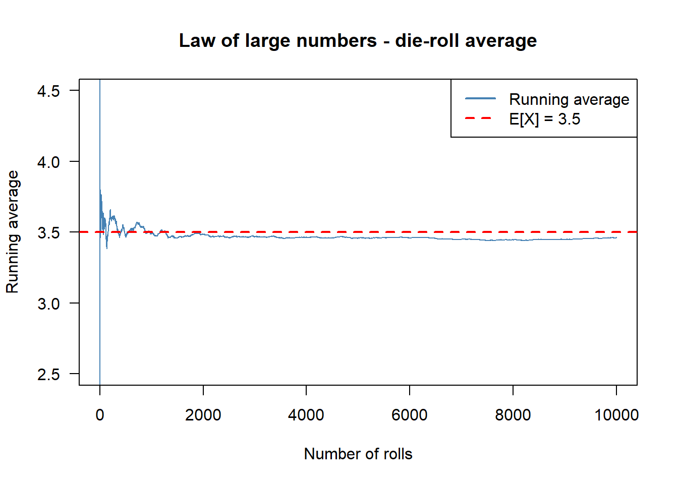

The running average wobbles wildly at first but settles tightly around 3.5 as $n$ grows.

4.10.2 Birthday paradox

Code

birthday_sim <- function(n_people, n_sim = 10000) {
  matches <- replicate(n_sim, {
    bdays <- sample(1:365, n_people, replace = TRUE)
    any(duplicated(bdays))
  })
  mean(matches)
}

p23 <- birthday_sim(23)
c(simulated = round(p23, 4), theoretical = 0.5073)

  simulated theoretical 
     0.5025      0.5073

Code

group_sizes <- 2:60
probs <- sapply(group_sizes, birthday_sim)
plot(group_sizes, probs, type = "l", col = "steelblue", lwd = 2,
     xlab = "Number of people", ylab = "P(at least one shared birthday)",
     main = "Birthday paradox", las = 1)
abline(h = 0.5, col = "red", lty = 2)
abline(v = 23, col = "grey50", lty = 3)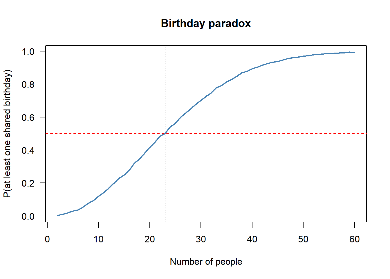

By 50 people a match is almost certain. The number of pairs grows as $\binom{n}{2}$ — quadratically, not linearly.

4.10.3 Conditional probability on cards

Code

suits <- rep(c("Hearts", "Diamonds", "Clubs", "Spades"), each = 13)
colors <- ifelse(suits %in% c("Hearts", "Diamonds"), "Red", "Black")
deck <- data.frame(Suit = suits, Color = colors, stringsAsFactors = FALSE)

draws <- deck[sample(52, n_sim, replace = TRUE), ]
red_draws <- draws[draws$Color == "Red", ]
c(sim = round(mean(red_draws$Suit == "Hearts"), 4),
  theory = round(13/26, 4))

   sim theory 
0.4954 0.5000

Half the red cards are hearts, so $P(\text{Heart} \mid \text{Red}) = 1/2$, confirming $P(A \mid B) = P(A \cap B)/P(B)$.

4.10.4 Bayes’ theorem: the medical test

Code

n_pop       <- 1e6
prevalence  <- 0.01
sensitivity <- 0.99
specificity <- 0.95

disease     <- rbinom(n_pop, 1, prevalence)
test_result <- ifelse(disease == 1,
                      rbinom(n_pop, 1, sensitivity),
                      rbinom(n_pop, 1, 1 - specificity))

conf <- table(Disease = factor(disease,     labels = c("No",  "Yes")),
              Test    = factor(test_result, labels = c("Neg", "Pos")))
conf

       Test
Disease    Neg    Pos
    No  940476  49473
    Yes    110   9941

Code

tp <- conf["Yes", "Pos"]; fp <- conf["No", "Pos"]
ppv_sim    <- tp / (tp + fp)
ppv_theory <- (sensitivity * prevalence) /
              (sensitivity * prevalence + (1 - specificity) * (1 - prevalence))
c(simulated = round(ppv_sim, 4), bayes = round(ppv_theory, 4))

simulated     bayes 
   0.1673    0.1667

Despite 99% sensitivity, a positive result corresponds to only about a 17% chance of disease — the base-rate fallacy in action.

4.10.5 Monty Hall

Code

simulate_monty <- function(n, strategy) {
  wins <- 0
  for (i in 1:n) {
    car  <- sample(1:3, 1)
    pick <- sample(1:3, 1)
    available  <- setdiff(1:3, c(pick, car))
    host_opens <- available[sample(length(available), 1)]
    final <- if (strategy == "switch") setdiff(1:3, c(pick, host_opens)) else pick
    if (final == car) wins <- wins + 1
  }
  wins / n
}

p_stay   <- simulate_monty(n_sim, "stay")
p_switch <- simulate_monty(n_sim, "switch")
c(stay = round(p_stay, 4), switch = round(p_switch, 4))

  stay switch 
0.3397 0.6530

Code

barplot(c(Stay = p_stay, Switch = p_switch),
        col = c("coral", "steelblue"), ylim = c(0, 0.8),
        main = "Monty Hall: stay vs switch", ylab = "Win probability", las = 1)
abline(h = c(1/3, 2/3), lty = 2, col = "grey50")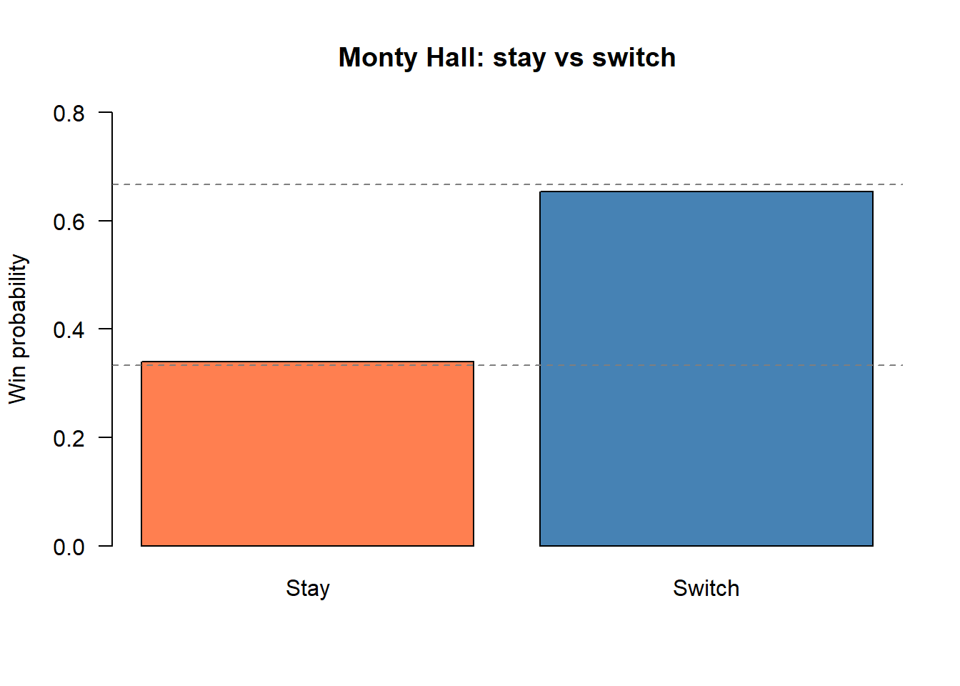

Switching wins roughly $2/3$ of the time, matching the Bayesian analysis above.

Self-check

Seven short multiple-choice questions. Try each one before opening the answer.

Q1. The Kolmogorov axioms

The Kolmogorov axioms require, for any event $A$ in the sample space $\Omega$, that:

A. $P(A) \in [-1, 1]$ and $P(\Omega) = 0$.
B. $P(A) \geq 0$, $P(\Omega) = 1$, and $P(A \cup B) = P(A) + P(B)$ when $A$ and $B$ are mutually exclusive.
C. $P(A) > 0$ for every event.
D. $P(A \cup B) = P(A) \cdot P(B)$ for any pair of events.

Answer: B. These are the three axioms — non-negativity, normalisation, and finite additivity for disjoint events.

Q2. Inclusion-exclusion

For two events $A$ and $B$, the formula $P(A \cup B) = P(A) + P(B) - P(A \cap B)$ subtracts $P(A \cap B)$ because:

A. Otherwise the intersection $A \cap B$ would be counted twice.
B. Probabilities must always sum to 1.
C. It corrects for non-negativity violations.
D. It is the definition of independence.

Answer: A. Adding $P(A)$ and $P(B)$ double-counts the overlap; subtracting $P(A \cap B)$ removes the duplication.

Q3. Independence

Two events $A$ and $B$ are independent if and only if:

A. $P(A \cap B) = P(A) \cdot P(B)$.
B. $P(A \cup B) = P(A) + P(B)$.
C. $A$ and $B$ are mutually exclusive.
D. $P(A \mid B) = 0$.

Answer: A. This is the definition. Option C describes mutual exclusivity, which is in fact incompatible with independence when both events have positive probability.

Q4. Conditional probability

The conditional probability of $A$ given $B$ (when $P(B) > 0$) is defined as:

A. $P(A \mid B) = P(A) / P(B)$.
B. $P(A \mid B) = P(A \cap B) / P(B)$.
C. $P(A \mid B) = P(A) \cdot P(B)$.
D. $P(A \mid B) = P(B \mid A)$ for any pair of events.

Answer: B. This is the textbook definition. Conditioning on $B$ rescales by the new sample space $B$.

Q5. Total probability and Bayes

Bayes’ theorem expands the denominator $P(B)$ via the law of total probability as:

A. $P(B) = P(B \mid A) P(A) + P(B \mid A^c) P(A^c)$.
B. $P(B) = P(B \mid A) + P(B \mid A^c)$.
C. $P(B) = P(A) + P(A^c)$.
D. $P(B) = 1 - P(A)$.

Answer: A. The partition is $\{A, A^c\}$; total probability adds the weighted conditional probabilities.

Q6. The base-rate fallacy

In the medical test example (sensitivity 99%, specificity 95%, prevalence 1%) the PPV is $P(D \mid +) \approx 0.17$. The intuition is:

A. With only 1% of the population sick, the 5% false-positive rate among the 99% healthy generates more false positives than true positives — the base rate dominates.
B. 99% sensitivity guarantees a 99% probability of disease given a positive test.
C. Specificity is irrelevant once prevalence is known.
D. The PPV equals sensitivity minus the false-positive rate.

Answer: A. The product (false-positive rate)$\times$(prevalence of healthy) is the dominant term when the disease is rare.

Q7. Monty Hall

In the Monty Hall problem (three doors, host opens a goat door after your first pick), switching wins with probability:

A. $1/2$, because two doors remain.
B. $1/3$, the same as staying.
C. $2/3$, because the host’s constrained action concentrates the remaining probability on the unopened door.
D. $1$, switching always wins.

Answer: C. The host’s behaviour is informative because he never opens your door and never opens the car door. The $2/3$ posterior collapses onto the door he leaves closed.

Exercises

4.10.6 Exercise 3.1 ★ — Set operations on a die

A fair die is rolled once. Define $A = \{1,2,3\}$, $B = \{3,4,5,6\}$, $C = \{2,4,6\}$. Compute:

$P(A \cup B)$.
$P(A \cap C)$.
$P(\bar{B} \cup C)$.
$P(A \cap B \cap C)$.
Are $A$ and $C$ independent?

Solution

$A \cup B = \Omega$ so $P(A \cup B) = 1$.
$A \cap C = \{2\}$ so $P(A \cap C) = 1/6$.
$\bar{B} = \{1,2\}$, $\bar{B} \cup C = \{1,2,4,6\}$, so $P(\bar{B} \cup C) = 4/6 = 2/3$.
$A \cap B = \{3\}$ and $\{3\} \cap C = \emptyset$, so $P(A \cap B \cap C) = 0$.
$P(A)P(C) = (1/2)(1/2) = 1/4 \ne 1/6 = P(A \cap C)$, so $A$ and $C$ are not independent.

4.10.7 Exercise 3.2 ★ — Laplace probability with a lottery

A regional chamber of commerce holds a lottery for 50 businesses: 20 retail shops, 15 restaurants, 10 tech companies, and 5 consulting firms.

What is the probability that the winner is a restaurant?
What is the probability that the winner is either a tech company or a consulting firm?
Two prizes are drawn without replacement. What is the probability that both winners are retail shops?

Solution

$P(\text{restaurant}) = 15/50 = 0.30$.
$P(\text{tech} \cup \text{consulting}) = 15/50 = 0.30$.
$P(\text{both retail}) = \dfrac{20}{50} \cdot \dfrac{19}{49} = \dfrac{380}{2450} \approx 0.155$.

4.10.8 Exercise 3.3 ★★ — Inclusion-exclusion in a tax registry

In a city of 10,000 taxpayers: 3,500 have self-employment income (event $A$), 5,200 have salaried income (event $B$), and 1,400 have both.

Compute $P(A \cup B)$.
What is the probability of having neither source of income?
Compute $P(A \cap \bar{B})$, the probability of self-employment income only.