---
title: "Formula Sheet and Exam Preparation"
---
> *Status: ported 2026-05-19. Reviewed by editor: pending.*
```{r appC-setup}
#| include: false
knitr::opts_chunk$set(echo = TRUE, warning = FALSE, message = FALSE,
fig.width = 8, fig.height = 4.5,
comment = "#>")
set.seed(2026)
options(scipen = 999)
```
::: {.callout-note}
## How to use this guide
Each topic has (1) a formula cheat sheet, (2) a *common mistakes* alert, (3) a quick decision rule, and (4) one fully solved exam-style exercise in R. Try the exercise on paper before unfolding the worked solution. Print this page for an offline reference.
:::
## C.1 — Topic 1: Univariate descriptive statistics
### Key formulas
| Measure | Formula | When to use |
|---------|---------|-------------|
| Arithmetic mean | $\bar{x} = \frac{1}{n}\sum x_i n_i$ | Symmetric data, no outliers |
| Median | $Me = L_i + \frac{n/2 - N_{i-1}}{n_i} \cdot a_i$ | Skewed data, outliers |
| Mode | Interval with highest $h_i = n_i / a_i$ | Categorical / grouped data |
| Variance ($S^2$, divisor $n$) | $S^2 = \frac{\sum x_i^2 n_i}{n} - \bar{x}^2$ | Always (primary dispersion) |
| Coefficient of variation | $CV = S / \bar{x}$ | Comparing across scales |
| Skewness | $g_1 = m_3 / S^3$ | Detect asymmetry |
| Kurtosis | $g_2 = m_4 / S^4 - 3$ | Tail heaviness |
| Gini index | $G = 1 - \sum(p_i - p_{i-1})(q_i + q_{i-1})$ | Inequality |
| Linear transform | If $Y = a + bX$: $\bar{y} = a + b\bar{x}$, $S_Y = \lvert b \rvert\, S_X$ | Currency, unit change |
### Decision rule
> **Which central-tendency measure?** Nominal $\to$ Mode. Ordinal $\to$ Median. Ratio/interval, symmetric $\to$ Mean. Skewed or outliers $\to$ Median.
::: {.callout-warning}
## Common mistakes (Topic 1)
1. **Using frequency as histogram height with unequal intervals.** Use density $h_i = n_i / a_i$.
2. **Forgetting class marks** ($c_i$, midpoints) for grouped data.
3. **Comparing variances across different scales.** Use $CV$ instead.
4. **Computing Gini without sorting** values from smallest to largest first.
5. **Confusing $S^2$ (divisor $n$) with $\hat{\sigma}^2$ (divisor $n-1$).** This course uses $S^2 = \frac{1}{n}\sum(x_i - \bar{x})^2$.
:::
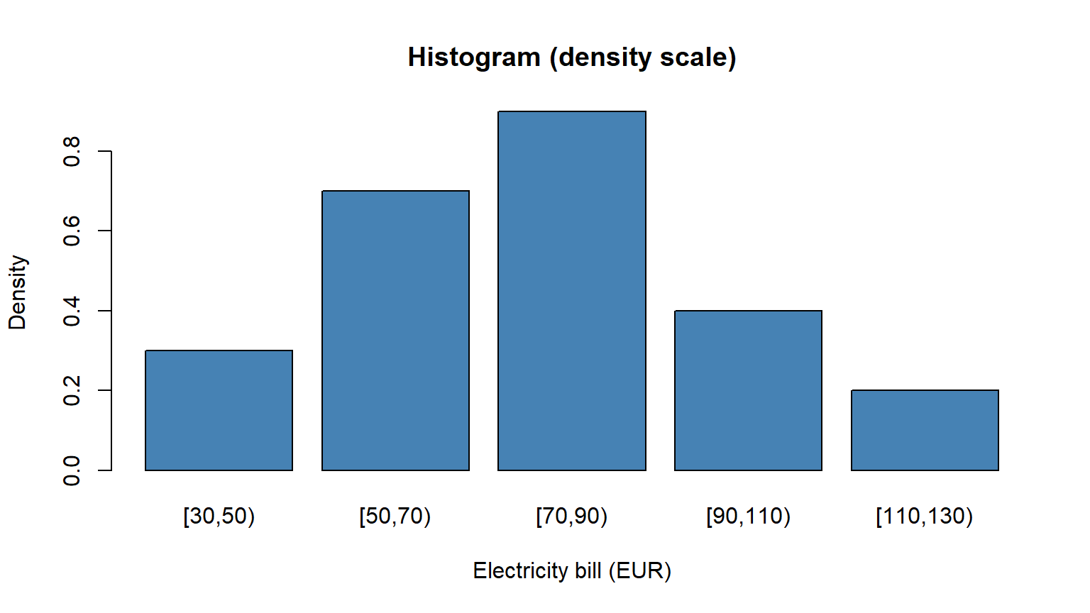
### Worked exam exercise — Monthly electricity bills
Monthly electricity bills (EUR) for 50 households are grouped into intervals $[30,50), [50,70), [70,90), [90,110), [110,130)$ with frequencies $n_i = 6, 14, 18, 8, 4$. Compute the mean, variance, $CV$, median, and skewness. Plot the density-scale histogram.
::: {.callout-tip collapse="true"}
## Solution
```{r appC-t1-exercise}
intervals <- c(30, 50, 70, 90, 110, 130)
ni <- c(6, 14, 18, 8, 4)
n  <- sum(ni)
ci <- (intervals[-length(intervals)] + intervals[-1]) / 2   # class marks
ai <- diff(intervals)                                       # widths

# Mean
x_bar <- sum(ci * ni) / n
cat("Mean =", round(x_bar, 2), "EUR\n")
# Variance and SD
S2 <- sum(ci^2 * ni) / n - x_bar^2
S  <- sqrt(S2)
cat("Variance =", round(S2, 2), ", SD =", round(S, 2), "\n")
# CV
CV <- S / x_bar
cat("CV =", round(CV, 4), "(", round(CV * 100, 1), "%)\n")
# Median
Ni <- cumsum(ni)
med_idx <- which(Ni >= n / 2)[1]
Me <- intervals[med_idx] + (n / 2 - c(0, Ni)[med_idx]) / ni[med_idx] * ai[med_idx]
cat("Median =", round(Me, 2), "EUR\n")
# Skewness
m3 <- sum(ni * (ci - x_bar)^3) / n
g1 <- m3 / S^3
cat("Skewness g1 =", round(g1, 3),
    ifelse(g1 > 0, "(right-skewed)",
           ifelse(g1 < 0, "(left-skewed)", "(symmetric)")), "\n")
# Histogram (density scale)
barplot(ni / ai,
        names.arg = paste0("[", intervals[-6], ",", intervals[-1], ")"),
        col = "steelblue", ylab = "Density", xlab = "Electricity bill (EUR)",
        main = "Histogram (density scale)")
```
**Interpretation.** The distribution is slightly right-skewed ($g_1 > 0$), so the mean exceeds the median. A $CV$ of about 30% indicates moderate dispersion.
:::
## C.2 — Topic 2: Bivariate descriptive statistics
### Key formulas
| Measure | Formula |
|---------|---------|
| Covariance | $S_{XY} = \overline{xy} - \bar{x}\bar{y}$ |
| Correlation | $r = S_{XY} / (S_X \cdot S_Y)$, always in $[-1, 1]$ |
| OLS slope | $b = S_{XY} / S_X^2$ |
| OLS intercept | $a = \bar{y} - b\bar{x}$ |
| Coefficient of determination | $R^2 = r^2$, fraction of variance explained |
| Statistical independence | $f_{ij} = f_{i\cdot} \cdot f_{\cdot j}$ for **all** $i, j$ |
| Exponential fit | $\log y = \log a + x \log b$; OLS on $(x, \log y)$ |
### Decision rule
> **Linear or nonlinear?** Plot first. Straight pattern $\to$ linear OLS. Curved and accelerating $\to$ exponential ($\log y$). Curved and decelerating $\to$ power ($\log x, \log y$). U-shape $\to$ quadratic.
::: {.callout-warning}
## Common mistakes (Topic 2)
1. **Confusing correlation with causation.** A high $r$ does not prove $X$ causes $Y$.
2. **Extrapolating beyond the data range.** The line is only meaningful within observed $x$ values.
3. **Only checking one cell for independence.** You must verify $f_{ij} = f_{i\cdot} f_{\cdot j}$ for *all* cells. One failure $\Rightarrow$ dependent.
4. **Reporting $R^2$ on log-transformed variables** as if it applied to the original scale.
5. **Forgetting that $b$ changes if you swap $X$ and $Y$.** The regression of $Y$ on $X$ is not the same as $X$ on $Y$.
:::
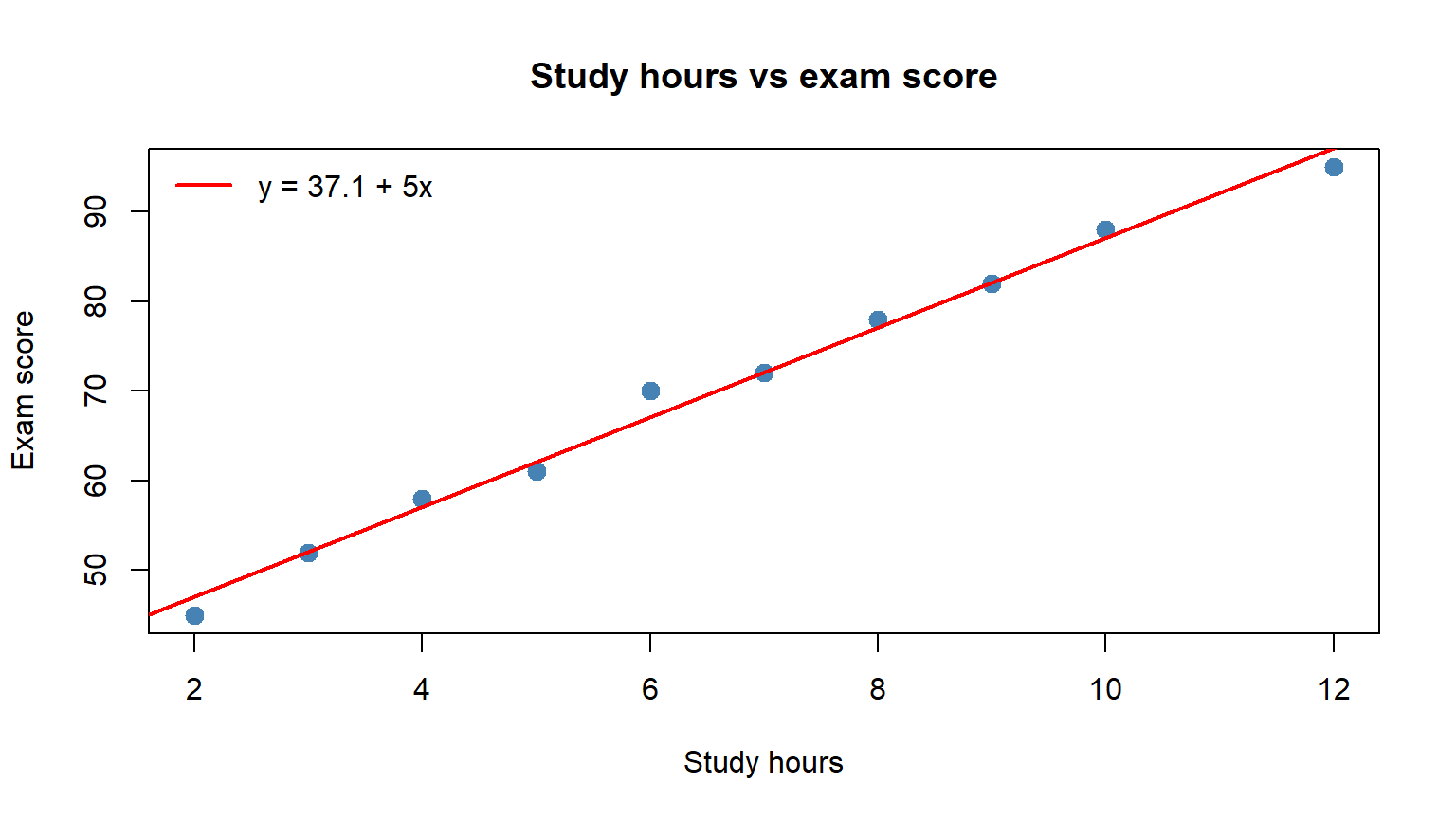
### Worked exam exercise — Study hours vs exam score
For ten students with study hours $x = (2,3,4,5,6,7,8,9,10,12)$ and scores $y = (45,52,58,61,70,72,78,82,88,95)$, compute $S_{XY}$, $S_X^2$, $S_Y^2$, the OLS line $y = a + bx$, the correlation $r$, $R^2$, and predict the score for 6.5 hours.
::: {.callout-tip collapse="true"}
## Solution
```{r appC-t2-exercise}
hours <- c(2, 3, 4, 5, 6, 7, 8, 9, 10, 12)
score <- c(45, 52, 58, 61, 70, 72, 78, 82, 88, 95)

# Scatter plot
plot(hours, score, pch = 19, col = "steelblue", cex = 1.3,
     xlab = "Study hours", ylab = "Exam score",
     main = "Study hours vs exam score")

# By-hand computation
n     <- length(hours)
x_bar <- mean(hours)
y_bar <- mean(score)
Sxy   <- mean(hours * score) - x_bar * y_bar
Sx2   <- mean(hours^2) - x_bar^2
Sy2   <- mean(score^2) - y_bar^2

b  <- Sxy / Sx2
a  <- y_bar - b * x_bar
r  <- Sxy / (sqrt(Sx2) * sqrt(Sy2))
R2 <- r^2

cat("x_bar =", x_bar, ", y_bar =", y_bar, "\n")
cat("Sxy =", round(Sxy, 3), ", Sx2 =", round(Sx2, 3), "\n")
cat("Slope b =", round(b, 3), "\n")
cat("Intercept a =", round(a, 3), "\n")
cat("r =", round(r, 4), ", R^2 =", round(R2, 4), "\n")
abline(a, b, col = "red", lwd = 2)
legend("topleft",
       legend = paste0("y = ", round(a, 1), " + ", round(b, 2), "x"),
       col = "red", lwd = 2, bty = "n")
# Verify with lm()
fit <- lm(score ~ hours)
cat("\nlm() verification:\n"); print(coef(fit))
cat("\nPredicted score for 6.5 hours:", round(a + b * 6.5, 1), "\n")
```
**Interpretation.** Each additional study hour increases the expected score by roughly `r round(b, 1)` points. With $R^2 \approx `r round(R2, 2)`$, study hours explain about `r round(R2 * 100)`% of score variability.
:::
## C.3 — Topic 3: Introduction to probability
### Key formulas
| Rule | Formula |
|------|---------|
| Complement | $P(\bar{A}) = 1 - P(A)$ |
| Addition | $P(A \cup B) = P(A) + P(B) - P(A \cap B)$ |
| Conditional | $P(A \mid B) = P(A \cap B) / P(B)$ |
| Product | $P(A \cap B) = P(A \mid B) \cdot P(B)$ |
| Independence | $P(A \cap B) = P(A) \cdot P(B)$ |
| Total probability | $P(B) = \sum_i P(B \mid A_i) P(A_i)$ |
| Bayes' theorem | $P(A_i \mid B) = \dfrac{P(B \mid A_i) P(A_i)}{\sum_j P(B \mid A_j) P(A_j)}$ |
### Decision rule
> **Which formula?** Single event $\to$ complement or Laplace. Two events $\to$ check independent vs mutually exclusive. Sequential events $\to$ tree diagram with the product rule. "Given that..." $\to$ conditional probability. "What caused the observed outcome?" $\to$ Bayes' theorem.
::: {.callout-warning}
## Common mistakes (Topic 3)
1. **Confusing independent and mutually exclusive.** Mutually exclusive events ($A \cap B = \emptyset$) are *dependent* — knowing $A$ occurred tells you $B$ did not.
2. **Applying Laplace's rule when outcomes are NOT equally likely** (loaded dice, biased coins).
3. **Ignoring base rates (the base-rate fallacy).** A 99%-accurate test on a rare disease still produces mostly false positives.
4. **Multiplying probabilities without checking independence.** $P(A \cap B) = P(A) P(B)$ holds only under independence.
5. **Forgetting that posteriors must sum to 1** after applying Bayes' theorem.
:::
### Worked exam exercise — Bayes' theorem (two factories)
Factory A supplies 60% of stock with a 3% defect rate; Factory B supplies 40% with a 7% defect rate. A defective item is found. Compute $P(\text{Defective})$, $P(A \mid D)$ and $P(B \mid D)$, and verify by simulation.
::: {.callout-tip collapse="true"}
## Solution
```{r appC-t3-exercise}
P_A   <- 0.60;  P_B   <- 0.40
P_D_A <- 0.03;  P_D_B <- 0.07

# Total probability of defect
P_D <- P_D_A * P_A + P_D_B * P_B
cat("P(D) =", P_D, "\n")
# Bayes
P_A_D <- (P_D_A * P_A) / P_D
P_B_D <- (P_D_B * P_B) / P_D
cat("P(A|D) =", round(P_A_D, 4), "\n")
cat("P(B|D) =", round(P_B_D, 4), "\n")
cat("Check: sum =", P_A_D + P_B_D, "\n")
# Monte-Carlo check
n_sim <- 100000
factory <- sample(c("A", "B"), n_sim, replace = TRUE, prob = c(0.60, 0.40))
defect  <- ifelse(factory == "A",
                  rbinom(n_sim, 1, 0.03),
                  rbinom(n_sim, 1, 0.07))
defectives <- factory[defect == 1]
cat("\nSimulation (", n_sim, "items):\n")
cat("P(A|D) simulated =", round(mean(defectives == "A"), 4), "\n")
cat("P(B|D) simulated =", round(mean(defectives == "B"), 4), "\n")
```
**Interpretation.** Although Factory A supplies 60% of stock, it is responsible for only about `r round(P_A_D * 100, 1)`% of defectives. Factory B, with its higher defect rate, is the more likely source.
:::
## C.4 — Topic 4: Random variables
### Key formulas
| Concept | Discrete | Continuous |
|---------|----------|------------|
| Mean | $\mu = \sum x_i p_i$ | $\mu = \int x f(x)\, dx$ |
| Variance | $\sigma^2 = \sum x_i^2 p_i - \mu^2$ | $\sigma^2 = \int x^2 f(x)\, dx - \mu^2$ |
| CDF | $F(x) = P(X \le x) = \sum_{x_i \le x} p_i$ | $F(x) = \int_{-\infty}^x f(t)\, dt$ |
| $P(a < X \le b)$ | $F(b) - F(a)$ | $\int_a^b f(x)\, dx$ |
| Linear transform | $\mathbb{E}[aX + b] = a\mu + b$ | $\operatorname{Var}(aX + b) = a^2 \sigma^2$ |
| Covariance | $\sigma_{XY} = \mathbb{E}[XY] - \mu_X \mu_Y$ | Independence $\Rightarrow \rho = 0$ (not vice versa) |
### Decision rule
> **Discrete or continuous?** Countable values (0, 1, 2, …) $\to$ discrete: use sums and PMF $p_i$. Uncountable values (an interval) $\to$ continuous: use integrals and density $f(x)$. For $\operatorname{Var}(X)$ always use $\mathbb{E}[X^2] - \mu^2$; for any linear function use $\mathbb{E}[aX + b] = a\mu + b$, $\operatorname{Var}(aX + b) = a^2 \sigma^2$.
::: {.callout-warning}
## Common mistakes (Topic 4)
1. **Forgetting that $P(X = a) = 0$ for continuous RVs.** Probability is area under $f$, not a height.
2. **Writing $\mathbb{E}[X^2] = (\mathbb{E}[X])^2$.** They are not equal; $\operatorname{Var}(X) = \mathbb{E}[X^2] - (\mathbb{E}[X])^2 \ge 0$.
3. **Assuming zero covariance implies independence.** $\rho = 0$ only rules out *linear* dependence.
4. **Forgetting to check that $\sum p_i = 1$** (or $\int f(x)\, dx = 1$) before computing expectations.
5. **Subtracting variances** when computing $\operatorname{Var}(X - Y)$. The correct formula is $\operatorname{Var}(X) + \operatorname{Var}(Y) - 2\operatorname{Cov}(X, Y)$.
:::
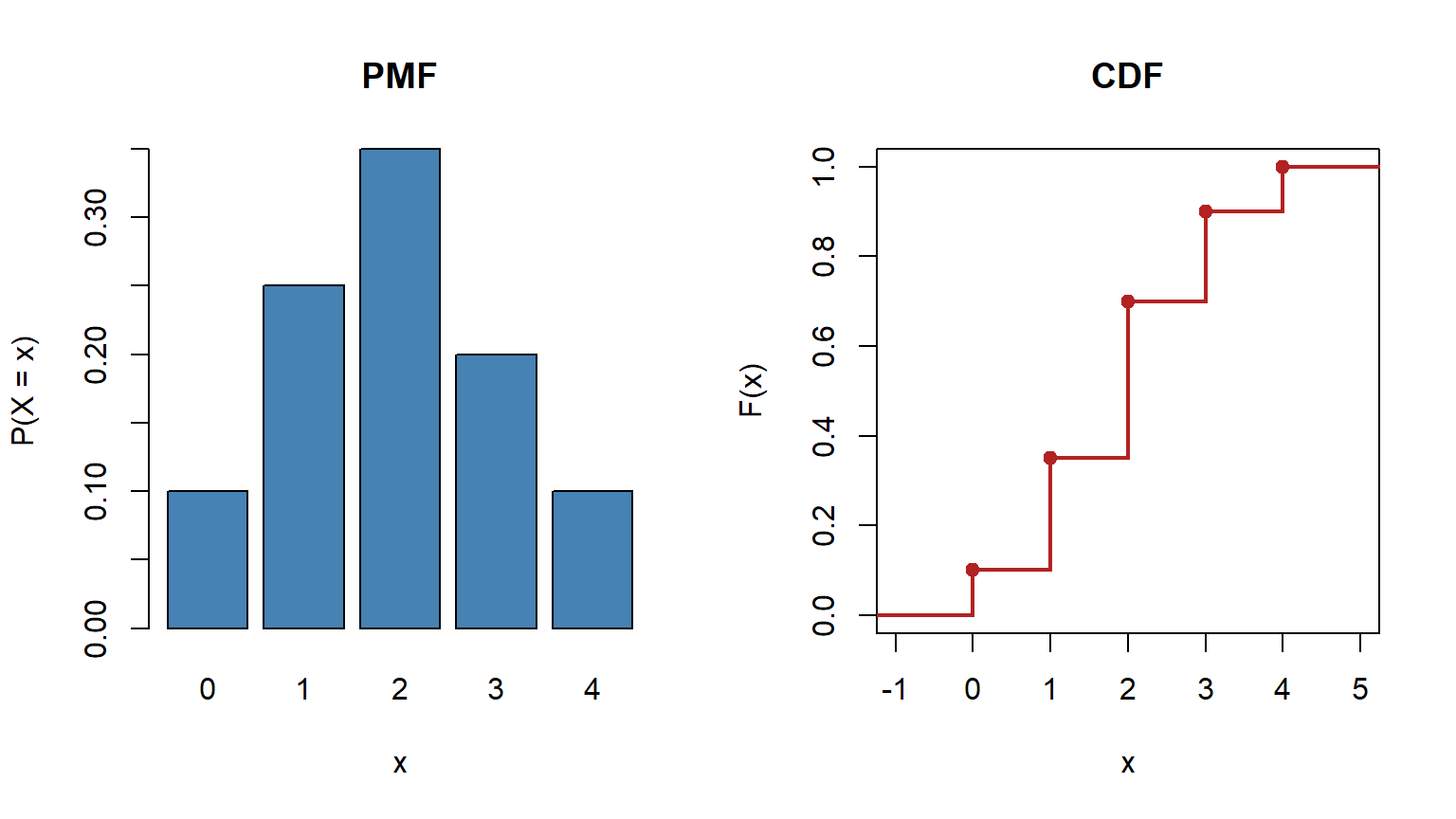
### Worked exam exercise — A discrete PMF
Let $X$ be daily product demand with PMF $P(X = x)$ given by $p = (0.10, 0.25, 0.35, 0.20, 0.10)$ on $x = 0, 1, 2, 3, 4$. Verify the PMF, compute $\mathbb{E}[X]$, $\mathbb{E}[X^2]$, $\operatorname{Var}(X)$, the CDF, and $P(1 \le X \le 3)$.
::: {.callout-tip collapse="true"}
## Solution
```{r appC-t4-exercise}
x <- c(0, 1, 2, 3, 4)
p <- c(0.10, 0.25, 0.35, 0.20, 0.10)

cat("Sum of probabilities:", sum(p), "\n")
EX   <- sum(x * p)
EX2  <- sum(x^2 * p)
VarX <- EX2 - EX^2
cat("E[X]   =", EX, "\n")
cat("E[X^2] =", EX2, "\n")
cat("Var(X) =", VarX, ", SD =", round(sqrt(VarX), 3), "\n")
# CDF
Fx <- cumsum(p)
knitr::kable(
  data.frame(x = x, `P(X=x)` = p, `F(x)` = Fx, check.names = FALSE),
  digits = 2)
cat("\nP(1 <= X <= 3) = F(3) - F(0) =", Fx[4] - Fx[1], "\n")
par(mfrow = c(1, 2))
barplot(p, names.arg = x, col = "steelblue",
        ylab = "P(X = x)", xlab = "x", main = "PMF")
plot(stepfun(x, c(0, Fx)), pch = 19, col = "firebrick", lwd = 2,
     main = "CDF", xlab = "x", ylab = "F(x)",
     xlim = c(-1, 5), ylim = c(0, 1))
par(mfrow = c(1, 1))
```
**Interpretation.** With $\mathbb{E}[X] = `r EX`$ and $\operatorname{Var}(X) = `r VarX`$, average daily demand is two units with standard deviation about `r round(sqrt(VarX), 2)`.
:::
## C.5 — Topic 5: Discrete distributions
### Key formulas
| Distribution | PMF | $\mu$ | $\sigma^2$ | Use when |
|--------------|-----|-------|-----------|----------|
| Binomial $B(n, p)$ | $\binom{n}{k} p^k (1-p)^{n-k}$ | $np$ | $np(1-p)$ | Fixed $n$ trials, constant $p$ |
| Poisson $\mathcal{P}(\lambda)$ | $\dfrac{e^{-\lambda}\lambda^k}{k!}$ | $\lambda$ | $\lambda$ | Counting events in an interval |
| Hypergeometric | $\dfrac{\binom{K}{k}\binom{N-K}{n-k}}{\binom{N}{n}}$ | $np$ | $np(1-p)\dfrac{N-n}{N-1}$ | Sampling without replacement |
| Geometric (failures) | $(1-p)^k p$ | $\dfrac{1-p}{p}$ | $\dfrac{1-p}{p^2}$ | Trials until the first success |
### Decision rule
> **Three questions to identify the distribution:**
>
> 1. Counting events in a fixed interval? $\to$ **Poisson**.
> 2. Waiting for the first success? $\to$ **Geometric**.
> 3. Fixed $n$ trials, count successes? With replacement $\to$ **Binomial**. Without replacement $\to$ **Hypergeometric**.
::: {.callout-warning}
## Common mistakes (Topic 5)
1. **Using Binomial when sampling WITHOUT replacement** from a small population. Use Hypergeometric.
2. **Confusing $P(X = k)$ with $P(X \le k)$.** "Exactly 3" vs "at most 3" vs "more than 3".
3. **Forgetting the Poisson rate adjustment.** If $\lambda = 3$ per hour and you want $P$ in two hours, use $\lambda' = 6$.
4. **Two conventions for the Geometric.** We count *failures before* the first success ($k = 0, 1, 2, \ldots$). Many textbooks count *trials until* success ($k = 1, 2, 3, \ldots$).
5. **Skipping the Poisson approximation conditions.** Rule of thumb: $n \ge 30$ and $p \le 0.10$.
:::
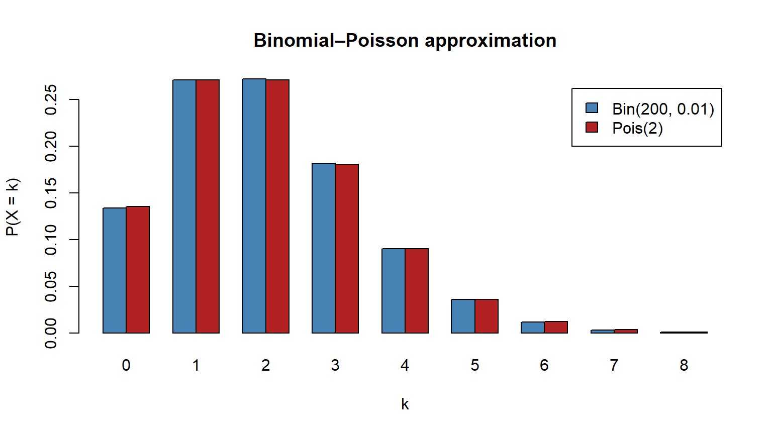
### Worked exam exercise — Poisson and Binomial-Poisson approximation
A bakery receives an average of $\lambda = 4$ complaints per week (Poisson). Compute $P(X = 0)$, $P(X \le 2)$, $P(X > 6)$. Then check the Poisson approximation to $B(200, 0.01)$ over $k = 0, \ldots, 8$.
::: {.callout-tip collapse="true"}
## Solution
```{r appC-t5-exercise}
lambda <- 4
cat("=== Poisson(lambda = 4) ===\n")
cat("P(X = 0) =", round(dpois(0, lambda), 4), "\n")
cat("P(X <= 2) =", round(ppois(2, lambda), 4), "\n")
cat("P(X > 6) =", round(1 - ppois(6, lambda), 4), "\n")
n <- 200; p_burn <- 0.01
cat("\n=== Binomial B(200, 0.01) vs Poisson(2) ===\n")
k        <- 0:8
binom_p  <- dbinom(k, n, p_burn)
pois_p   <- dpois(k, n * p_burn)
comparison <- data.frame(k = k,
                         Binomial   = round(binom_p, 5),
                         Poisson    = round(pois_p, 5),
                         Difference = round(binom_p - pois_p, 5))
knitr::kable(comparison)
barplot(rbind(binom_p, pois_p), beside = TRUE, names.arg = k,
        col = c("steelblue", "firebrick"),
        legend.text = c("Bin(200, 0.01)", "Pois(2)"),
        xlab = "k", ylab = "P(X = k)",
        main = "Binomial–Poisson approximation")
```
**Interpretation.** The approximation is excellent — the bars are visually indistinguishable, and the maximum difference is below 0.001.
:::
## C.6 — Topic 6: Index numbers
### Key formulas
| Index | Formula | Interpretation |
|-------|---------|---------------|
| Elementary | $I_{t/0} = \frac{Y_t}{Y_0} \times 100$ | Single-variable change |
| Laspeyres (price) | $L_P = \frac{\sum p_t q_0}{\sum p_0 q_0} \times 100$ | Cost of *old* basket at new prices |
| Paasche (price) | $P_P = \frac{\sum p_t q_t}{\sum p_0 q_t} \times 100$ | Cost of *current* basket comparison |
| Fisher | $F = \sqrt{L_P \times P_P}$ | Geometric-mean compromise |
| Laspeyres (quantity) | $L_Q = \frac{\sum q_t p_0}{\sum q_0 p_0} \times 100$ | Real consumption change |
| Value decomposition | $V = L_P \cdot P_Q / 100 = P_P \cdot L_Q / 100$ | Price + quantity effects |
| Deflation | $Y^{\text{real}} = Y^{\text{nominal}} / (\text{CPI}/100)$ | Remove inflation |
| Linking | $I_{t/\text{new}} = I_{t/\text{old}} / I_{\text{new}/\text{old}} \times 100$ | Change base period |
| Average growth rate | $\bar{T} = (Y_T/Y_0)^{1/T} - 1$ | Geometric mean of factors |
### Decision rule
> **Which weights do I use?** Price index with base-period quantities $\to$ Laspeyres. Price index with current-period quantities $\to$ Paasche. Need a symmetric compromise $\to$ Fisher. To remove inflation, divide nominal by $\text{CPI}/100$. To rebase to a new period, divide all values by $I_{\text{new}/\text{old}}$ and multiply by 100.
::: {.callout-warning}
## Common mistakes (Topic 6)
1. **Averaging rates of variation arithmetically.** Use the geometric mean of the *factors*, not the arithmetic mean of the rates.
2. **Dividing by the CPI instead of $\text{CPI}/100$** when deflating. If CPI = 115, divide by 1.15.
3. **Confusing Laspeyres and Paasche weights.** Laspeyres uses base-period quantities; Paasche uses current-period quantities.
4. **Forgetting to verify the value decomposition.** Always check $V = L_P \cdot P_Q / 100$.
5. **Applying the wrong linking formula.** To convert old base to new: divide by $I_{\text{new}/\text{old}}$ and multiply by 100.
:::
### Worked exam exercise — Three-good basket and deflation
Three goods (bread, milk, eggs) have base-period prices and quantities $p_0 = (1.20, 0.90, 2.50)$, $q_0 = (100, 200, 50)$ and current values $p_t = (1.50, 1.10, 2.80)$, $q_t = (90, 210, 45)$. Compute $L_P$, $P_P$, Fisher $F$, $L_Q$, $P_Q$, the value index $V$, and verify the decomposition. Then deflate a five-year nominal series with the given CPI.
::: {.callout-tip collapse="true"}
## Solution
```{r appC-t6-exercise}
goods <- c("Bread (kg)", "Milk (L)", "Eggs (dozen)")
p0 <- c(1.20, 0.90, 2.50);  q0 <- c(100, 200, 50)
pt <- c(1.50, 1.10, 2.80);  qt <- c(90, 210, 45)

basket <- data.frame(Good = goods, p0, q0, pt, qt,
                     p0q0 = p0 * q0, ptq0 = pt * q0,
                     p0qt = p0 * qt, ptqt = pt * qt)
knitr::kable(basket, digits = 1)
Lp <- sum(pt * q0) / sum(p0 * q0) * 100
Pp <- sum(pt * qt) / sum(p0 * qt) * 100
Fp <- sqrt(Lp * Pp)
Lq <- sum(qt * p0) / sum(q0 * p0) * 100
Pq <- sum(qt * pt) / sum(q0 * pt) * 100
V  <- sum(pt * qt) / sum(p0 * q0) * 100

cat("Laspeyres price =", round(Lp, 2), "\n")
cat("Paasche price =", round(Pp, 2), "\n")
cat("Fisher price =", round(Fp, 2), "\n")
cat("Laspeyres qty =", round(Lq, 2), "\n")
cat("Paasche qty =", round(Pq, 2), "\n")
cat("Value index =", round(V, 2), "\n")
cat("\nDecomposition check:\n")
cat(" Lp * Pq / 100 =", round(Lp * Pq / 100, 2), "\n")
cat(" Pp * Lq / 100 =", round(Pp * Lq / 100, 2), "\n")
cat(" Value index =", round(V, 2), "\n")
# Deflation example
cat("\n=== Deflation ===\n")
years   <- 2020:2024
nominal <- c(1500, 1560, 1620, 1700, 1800)
cpi     <- c(100, 103, 108, 115, 121)
real    <- nominal / (cpi / 100)
knitr::kable(data.frame(Year = years, Nominal = nominal,
                        CPI = cpi, Real = round(real, 1)))
cat("Nominal growth:", round((1800 / 1500 - 1) * 100, 1), "%\n")
cat("Real growth :", round((real[5] / real[1] - 1) * 100, 1), "%\n")
```
**Interpretation.** The value index decomposes exactly into either Laspeyres-price × Paasche-quantity or Paasche-price × Laspeyres-quantity (over 100). After deflating, real growth is markedly lower than nominal — most of the headline increase reflects inflation, not real gain.
:::
## C.7 — Topic 7: Time series
### Key formulas
| Step | Multiplicative model | Additive model |
|------|----------------------|----------------|
| Model | $Y_t = T_t \cdot E_t \cdot \varepsilon_t$ | $Y_t = T_t + E_t + \varepsilon_t$ |
| OLS trend | $\hat{T}_t = a + b t$ | same |
| Trend per season | $b / s$ | same |
| Seasonal index | $\text{IVE}_i = \dfrac{\operatorname{avg}(Y_t / \hat{T}_t)}{\text{global avg}}$ | $E_i = \operatorname{avg}(Y_t - \hat{T}_t)$, normalised to sum to 0 |
| Deseasonalised | $Y^* = Y_t / \text{IVE}_t$ | $Y^* = Y_t - E_t$ |
| Forecast | $\hat{Y}_t = \hat{T}_t \cdot \text{IVE}_t$ | $\hat{Y}_t = \hat{T}_t + E_t$ |
### Decision rule
> **Additive or multiplicative?** Plot the data. Constant seasonal swings $\to$ **Additive**. Swings grow with the trend $\to$ **Multiplicative**.
::: {.callout-warning}
## Common mistakes (Topic 7)
1. **Forgetting to centre the MA(4).** Even-order moving averages fall between time points and must be centred.
2. **Seasonal indices not normalised.** They must sum to $s$ (multiplicative) or to 0 (additive). If not, rescale.
3. **Confusing annual trend with per-season trend.** If $b$ is per year and the data are quarterly, trend per quarter $= b/4$.
4. **Forecasting too far ahead.** Univariate decomposition assumes the past pattern continues.
5. **Mixing additive IVEs with a multiplicative model (or vice versa).** Constant amplitude $\to$ additive; growing amplitude $\to$ multiplicative.
:::
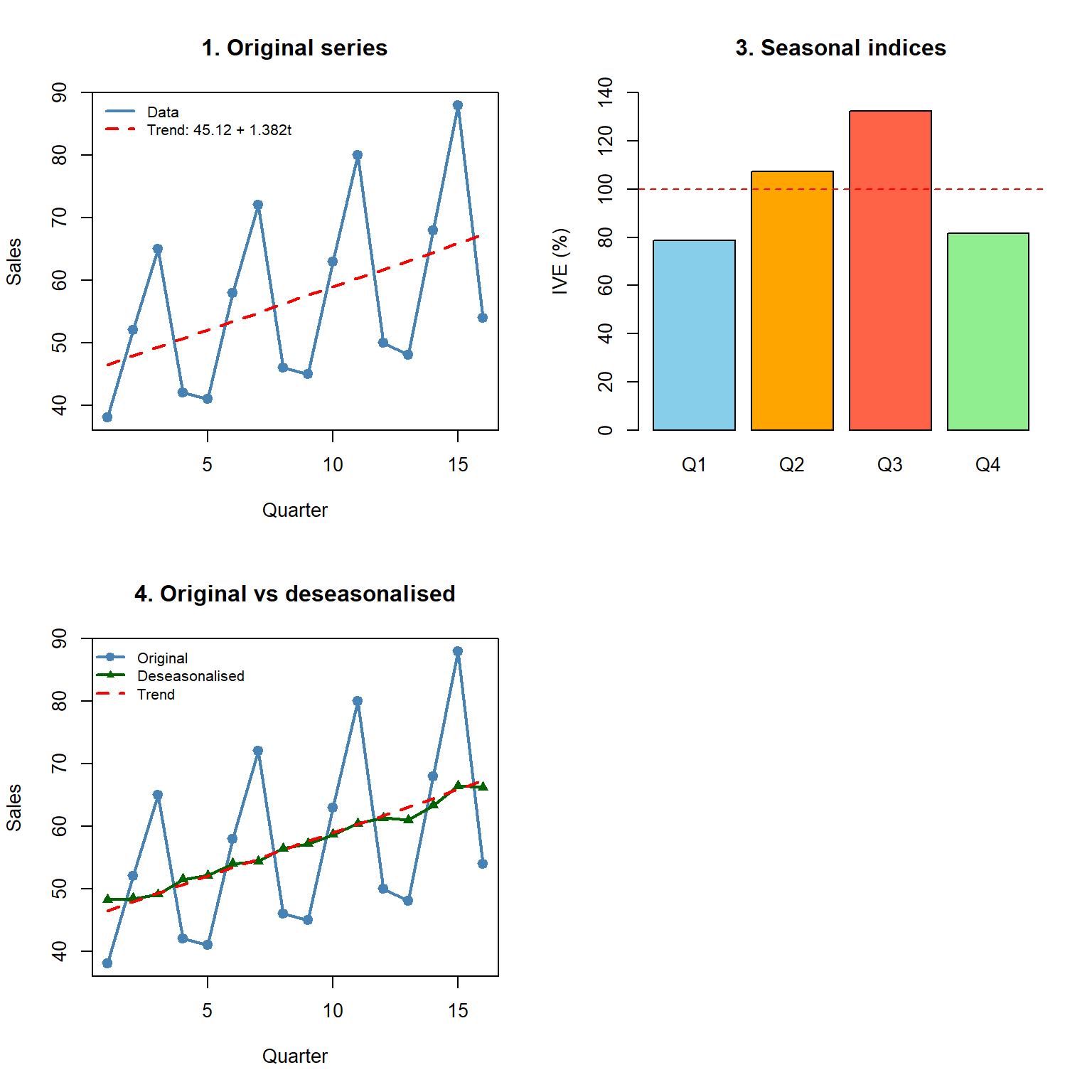
### Worked exam exercise — Full multiplicative decomposition
For quarterly sales over 4 years (2020–2023) given by $Y_t = (38, 52, 65, 42; 41, 58, 72, 46; 45, 63, 80, 50; 48, 68, 88, 54)$, fit an OLS trend, compute the multiplicative seasonal indices $\text{IVE}_i$ (Q1–Q4), deseasonalise, and forecast 2024.
::: {.callout-tip collapse="true"}
## Solution
```{r appC-t7-exercise}
#| fig-height: 8
t_idx <- 1:16
sales <- c(38, 52, 65, 42,   41, 58, 72, 46,
           45, 63, 80, 50,   48, 68, 88, 54)

par(mfrow = c(2, 2))

# 1. Plot
plot(t_idx, sales, type = "o", pch = 19, col = "steelblue", lwd = 2,
     xlab = "Quarter", ylab = "Sales", main = "1. Original series")

# 2. OLS trend
fit   <- lm(sales ~ t_idx)
trend <- fitted(fit)
a <- round(coef(fit)[1], 2); b <- round(coef(fit)[2], 3)
lines(t_idx, trend, col = "red", lwd = 2, lty = 2)
legend("topleft",
       c("Data", paste0("Trend: ", a, " + ", b, "t")),
       col = c("steelblue", "red"), lwd = 2, lty = c(1, 2),
       bty = "n", cex = 0.8)
cat("Trend: T =", a, "+", b, "* t\n")
cat("Trend per quarter:", round(b, 3), "\n\n")
# 3. Seasonal indices
ratio       <- sales / trend
ratio_mat   <- matrix(ratio, ncol = 4, byrow = TRUE)
colnames(ratio_mat) <- paste0("Q", 1:4)
avg_ratio   <- colMeans(ratio_mat)
global_mean <- mean(avg_ratio)
IVE         <- avg_ratio / global_mean

cat("Average ratios:", round(avg_ratio, 4), "\n")
cat("IVE :", round(IVE, 4), "\n")
cat("Sum of IVE :", round(sum(IVE), 4), "(should be 4)\n\n")
barplot(IVE * 100, names.arg = paste0("Q", 1:4),
        col = c("skyblue", "orange", "tomato", "lightgreen"),
        ylab = "IVE (%)", main = "3. Seasonal indices", ylim = c(0, 140))
abline(h = 100, lty = 2, col = "red")

# 4. Deseasonalise
deseas <- sales / rep(IVE, 4)
plot(t_idx, sales, type = "o", pch = 19, col = "steelblue", lwd = 2,
     xlab = "Quarter", ylab = "Sales",
     main = "4. Original vs deseasonalised")
lines(t_idx, deseas, type = "o", pch = 17, col = "darkgreen", lwd = 2)
lines(t_idx, trend, col = "red", lwd = 2, lty = 2)
legend("topleft", c("Original", "Deseasonalised", "Trend"),
       col = c("steelblue", "darkgreen", "red"),
       pch = c(19, 17, NA), lwd = 2, lty = c(1, 1, 2),
       bty = "n", cex = 0.8)

# 5. Forecast 2024
t_fc     <- 17:20
trend_fc <- a + b * t_fc
forecast <- trend_fc * IVE

cat("=== 2024 forecasts ===\n")
fc_df <- data.frame(Quarter  = paste0("Q", 1:4),
                    Trend    = round(trend_fc, 2),
                    IVE      = round(IVE, 4),
                    Forecast = round(forecast, 1))
knitr::kable(fc_df)
par(mfrow = c(1, 1))
```
**Interpretation.** Q3 is the peak season (IVE $\approx$ `r round(IVE[3] * 100, 1)`%, about `r round((IVE[3] - 1) * 100)`% above trend); Q1 is the weakest. The deseasonalised series tracks the linear trend closely, supporting the multiplicative model.
:::
## C.8 Notation bridge
Notation used across all seven topics.
| Concept | Descriptive (T1–T2) | Probabilistic (T4–T5) | Time series (T7) |
|---------|---------------------|------------------------|-------------------|
| Mean | $\bar{x}$ | $\mu = \mathbb{E}[X]$ | $\hat{T}_t$ (trend) |
| Variance | $S^2$ | $\sigma^2 = \operatorname{Var}(X)$ | — |
| Std deviation | $S$ | $\sigma$ | — |
| Covariance | $S_{XY}$ | $\sigma_{XY} = \operatorname{Cov}(X, Y)$ | — |
| Correlation | $r$ | $\rho = \operatorname{Corr}(X, Y)$ | — |
| Relative frequency | $f_i$ | $p_i$ (probability) | — |
| Cum. relative frequency | $F_i$ | $F(x)$ (CDF) | — |
## C.9 Final checklist
Before the exam, make sure you can:
- Build a frequency table from raw data and compute *all* descriptive statistics.
- Interpret the $CV$ to compare dispersion across different scales.
- Compute a regression line by hand and interpret slope, intercept, and $R^2$.
- Explain why correlation $\neq$ causation with a concrete example.
- Apply Bayes' theorem using a tree diagram or a $2 \times 2$ frequency table.
- Identify the correct probability distribution from a problem description.
- Compute Laspeyres, Paasche, and Fisher indices and interpret the decomposition.
- Deflate a nominal series using the CPI.
- Carry out a complete time-series decomposition (trend $\to$ IVE $\to$ deseasonalise $\to$ forecast).
- Explain the difference between additive and multiplicative models.