---
title: "The Simple Linear Regression Model"
---
## Learning outcomes {.unnumbered}
By the end of this chapter the reader should be able to:
- Write the population regression function (PRF) and the sample regression function (SRF) for the simple linear model, and explain what each one represents.
- Derive the OLS estimators $\hat\beta_0$ and $\hat\beta_1$ as the minimisers of the sum of squared residuals.
- State the five Gauss--Markov assumptions for the simple linear regression (SLR) model and explain what each one guarantees.
- Prove (or follow the proof of) the unbiasedness of OLS and identify which assumptions are used at each step.
- Write down the sampling variance of $\hat\beta_1$, name the three factors that drive its precision, and explain what BLUE means.
- Decompose total variation into $\mathrm{SST} = \mathrm{SSE} + \mathrm{SSR}$ and compute and interpret $R^2$.
- Use `lm()` in R to estimate, interpret, and visualise a simple regression on the `beauty` and `bwght` datasets.
## Motivating empirical question {.unnumbered}
> *How much higher is the wage of a worker rated "above average" in physical appearance, compared with a worker rated "average"?*
The labour-economics literature [@wooldridge2020] has long documented a "beauty premium" --- workers who are rated as more physically attractive tend to earn higher wages. Whether the premium is causal (looks open doors) or driven by confounding (looks correlate with health, social skills, family background) is a separate question. Before we can even *ask* that question we need a tool that turns a cloud of points into a single number. That tool is the **simple linear regression** of wage on a measure of looks. In §2.11 we estimate exactly this regression on Hamermesh's `beauty` dataset.
## Introduction
`\lettrine[lines=3]{R}{egression}`{=latex} analysis investigates the relationship between two or more variables. In this chapter we focus on the **simple linear regression** model (SLR), which relates a dependent variable $y$ to a single independent variable $x$:
$$
y = \beta_0 + \beta_1 x + u.
$$
Here $y$ is the dependent variable, $x$ is the independent variable (also called the regressor or explanatory variable), $\beta_0$ is the **intercept**, $\beta_1$ is the **slope**, and $u$ is the unobservable **error term** or *disturbance*, which collects every determinant of $y$ that is not $x$ [@wooldridge2020]. The slope parameter $\beta_1$ measures the change in $y$ associated with a one-unit change in $x$, *holding all factors in $u$ constant*:
$$
\beta_1 = \frac{\Delta y}{\Delta x} \quad \text{when } \Delta u = 0.
$$
The intercept $\beta_0$ is the value of $y$ when $x = 0$. In many applications $x = 0$ is outside the range of the data (zero years of education, zero square feet, zero cigarettes per day for a non-smoker) and the intercept has no immediate economic meaning --- it is still essential for the line to be in the right place.
::: {.callout-note}
## A small zoo of SLR examples
Each of the following is a simple linear regression of one outcome on one regressor. We will revisit several of them throughout the chapter.
- Wages on years of education: $\widehat{\text{Wage}} = 800 + 15\cdot\text{Educ}$. Each extra year of schooling is associated with an extra 15 euros per month, on average.
- House price on square footage: $\widehat{\text{Price}} = 100{,}000 + 50\cdot\text{SqFt}$.
- Car resale value on age: $\widehat{\text{Resale}} = 30{,}000 - 1{,}500\cdot\text{YearsOld}$.
- Sales on advertising spend: $\widehat{\text{Sales}} = 50 + 2\cdot\text{AdSpend}$.
- Blood pressure on age: $\widehat{\text{BP}} = 100 + 0.5\cdot\text{Age}$.
:::
## The population regression function
The model $y = \beta_0 + \beta_1 x + u$ involves the unobservable disturbance $u$. To turn it into a statement we can in principle test, we impose a key assumption on the conditional mean of the error:
$$
\mathbb{E}[u \mid x] = 0.
$$
This says that whatever determinants of $y$ are bundled into $u$, they are unrelated *on average* to $x$. Taking conditional expectations of both sides of the model and using this assumption yields the **population regression function (PRF)**:
$$
\mathbb{E}[y \mid x] = \beta_0 + \beta_1 x.
$$
The PRF describes the *average* value of $y$ at each value of $x$ in the population. It is a straight line with intercept $\beta_0$ and slope $\beta_1$.
::: {.callout-note}
## Regression is a comparison
Read $\beta_1$ as a *comparison between sub-populations*. If we compare the group of individuals with $x = a$ to the group with $x = a + 1$, the latter group has a value of $y$ that is on average $\beta_1$ units higher. Whether that comparison reflects a causal effect depends on whether $\mathbb{E}[u \mid x] = 0$ holds --- a question we keep coming back to throughout the book.
:::
The fundamental problem with the PRF is that it **cannot be observed**. It is a statement about an entire population that we never see. The best we can do is take a sample and estimate the line that, on the available evidence, comes closest to the truth.
::: {.callout-warning}
## Common mistake: confusing the PRF with the SRF
The PRF $\mathbb{E}[y \mid x] = \beta_0 + \beta_1 x$ is a property of the *population*: $\beta_0$ and $\beta_1$ are fixed but unknown. The SRF $\hat y = \hat\beta_0 + \hat\beta_1 x$ (next section) is a *random* line whose intercept and slope change from sample to sample. Confusing the two is the single most common conceptual error in this course.
:::
## The sample regression function
Let $\{(x_i, y_i) : i = 1, 2, \ldots, n\}$ be a random sample of size $n$ from the population. For each observation $i$ the population model is
$$
y_i = \beta_0 + \beta_1 x_i + u_i.
$$
We define the **sample regression function (SRF)** as
$$
\hat y_i = \hat\beta_0 + \hat\beta_1 x_i,
$$
where $\hat\beta_0$ and $\hat\beta_1$ are **estimates** of the population parameters $\beta_0$ and $\beta_1$, obtained from the data. The hats remind us at every step that these are sample-based quantities. Two different samples from the same population would, in general, yield two different SRFs.
## Ordinary Least Squares (OLS)
Given a scatter plot of $(x_i, y_i)$ data points, infinitely many lines could be drawn through the cloud, each with a different $(\hat\beta_0, \hat\beta_1)$. How do we choose the "best" line?
### Why we need a criterion {.unnumbered}
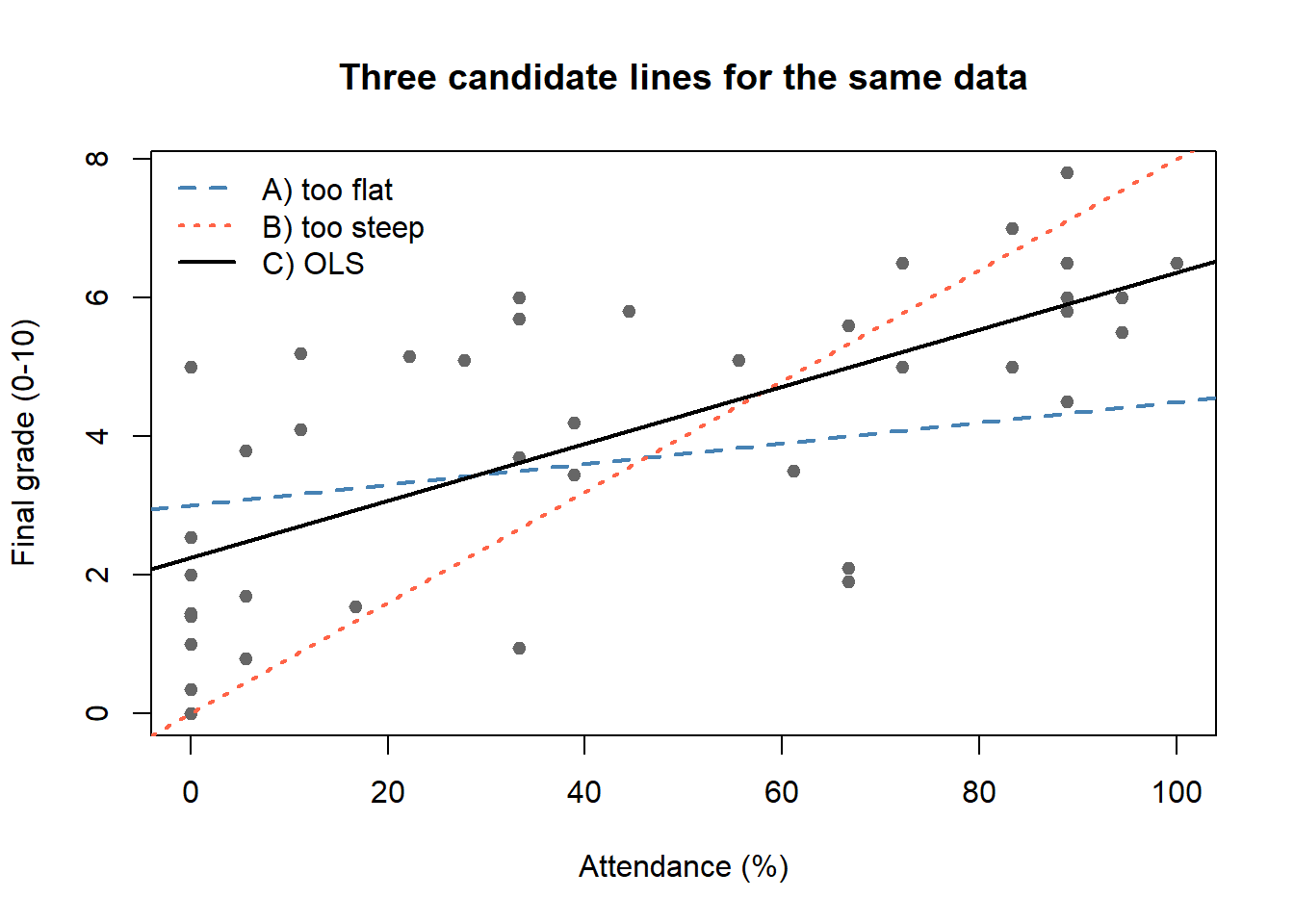
Here is a scatter plot of 41 students from a recent UGR Econometrics I cohort, plotting their attendance rate against their final grade. Many lines look like they could "roughly" fit the cloud of points; the question is which one we choose, and why. Before deriving any formulas, it helps to *see* the problem.
```{r slr-ols-criterion-fig}
# 41 students, UGR Econometrics I 2024-25 cohort
asistencia <- c(38.89, 94.44, 94.44, 33.33, 83.33, 0, 0, 66.67, 88.89,
                66.67, 27.78, 83.33, 0, 61.11, 0, 22.22, 0, 0, 72.22,
                88.89, 88.89, 11.11, 5.56, 33.33, 16.67, 0, 11.11,
                33.33, 100, 38.89, 5.56, 72.22, 44.44, 0, 55.56, 33.33,
                0, 66.67, 5.56, 88.89, 88.89)
nota       <- c(3.45, 5.5, 6, 3.7, 7, 2.55, 5, 2.1, 5.8, 1.9, 5.1, 5,
                2, 3.5, 2, 5.15, 0.35, 1.45, 5, 4.5, 7.8, 5.2, 3.8, 6,
                1.55, 1, 4.1, 5.7, 6.5, 4.2, 0.8, 6.5, 5.8, 0, 5.1,
                0.95, 1.4, 5.6, 1.7, 6.5, 6)

# Three candidate lines (we will compute their SSRs)
candidates <- data.frame(
  label = c("A) too flat", "B) too steep", "C) OLS"),
  b0    = c(3.0, 0.0, 2.256),
  b1    = c(0.015, 0.08, 0.0411)
)

# Scatter + the three candidate lines
plot(asistencia, nota,
     xlab = "Attendance (%)", ylab = "Final grade (0-10)",
     pch = 19, col = "grey40", cex = 0.9,
     main = "Three candidate lines for the same data")
cols <- c("steelblue", "tomato", "black")
ltys <- c(2, 3, 1)
for (k in seq_len(nrow(candidates))) {
  abline(a = candidates$b0[k], b = candidates$b1[k],
         col = cols[k], lwd = 2, lty = ltys[k])
}
legend("topleft", legend = candidates$label,
       col = cols, lty = ltys, lwd = 2, bty = "n")
# SSR for each candidate
ssr <- sapply(seq_len(nrow(candidates)), function(k) {
  yhat <- candidates$b0[k] + candidates$b1[k] * asistencia
  sum((nota - yhat)^2)
})
data.frame(line  = candidates$label,
           beta0 = candidates$b0,
           beta1 = candidates$b1,
           SSR   = round(ssr, 2))
```
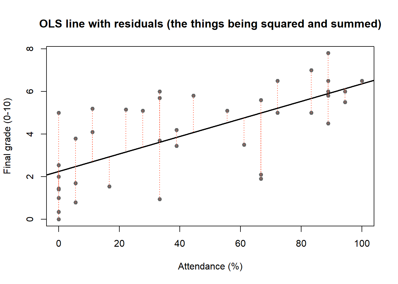
Each candidate line gives a different sum of squared residuals (SSR). OLS is the *unique* pair $(\hat\beta_0, \hat\beta_1)$ that minimises this sum --- line C above. The next figure shows the residuals (the very quantities being squared and summed) as dashed vertical segments from each point to the OLS line.
```{r slr-ols-residuals-fig}
m <- lm(nota ~ asistencia)
plot(asistencia, nota,
     xlab = "Attendance (%)", ylab = "Final grade (0-10)",
     pch = 19, col = "grey40", cex = 0.9,
     main = "OLS line with residuals (the things being squared and summed)")
abline(m, col = "black", lwd = 2)
yhat <- predict(m)
segments(asistencia, nota, asistencia, yhat,
         col = "tomato", lty = 3)
```
The formal definition of the residual $\hat u_i$ follows in §2.4.1; the algebraic derivation of the minimisers $\hat\beta_0$ and $\hat\beta_1$ follows in §2.4.3. The visual intuition stays with us: OLS is the line that makes the sum of squared dashed segments as small as possible.
::: {.callout-note appearance="simple"}
*Data: 41 estudiantes de Econometría I, curso 2024--25, UGR (recogidos por el autor).*
:::
### The residual
For each observation $i$, the **residual** is the vertical distance between the observed $y_i$ and the value predicted by the SRF:
$$
\hat u_i = y_i - \hat y_i = y_i - \hat\beta_0 - \hat\beta_1 x_i.
$$
The residual is the sample analogue of the population disturbance $u_i$. It is observable as soon as we have estimates $(\hat\beta_0, \hat\beta_1)$; the disturbance $u_i$ is *never* observable.
### The sum of squared residuals
We want the line that makes the residuals as small as possible in some overall sense. Squaring (rather than taking absolute values) penalises large deviations more heavily and yields a smooth, differentiable objective. The OLS method chooses $\hat\beta_0$ and $\hat\beta_1$ to minimise the **sum of squared residuals**:
$$
\mathrm{SSR} = \sum_{i=1}^{n} \hat u_i^{\,2} = \sum_{i=1}^{n}\bigl(y_i - \hat\beta_0 - \hat\beta_1 x_i\bigr)^2.
$$
### Derivation of the OLS estimators
Differentiating $\mathrm{SSR}$ with respect to $\hat\beta_0$ and $\hat\beta_1$ and setting the derivatives to zero gives the *first-order conditions* (FOCs):
$$
-2\sum_{i=1}^{n}\bigl(y_i - \hat\beta_0 - \hat\beta_1 x_i\bigr) = 0, \qquad
-2\sum_{i=1}^{n} x_i\bigl(y_i - \hat\beta_0 - \hat\beta_1 x_i\bigr) = 0.
$$
The first FOC, divided by $n$, gives $\bar y - \hat\beta_0 - \hat\beta_1 \bar x = 0$, hence
$$
\hat\beta_0 = \bar y - \hat\beta_1 \bar x.
$$
Substituting this back into the second FOC and simplifying yields the celebrated formula for the slope:
$$
\hat\beta_1 = \frac{\sum_{i=1}^{n}(x_i - \bar x)(y_i - \bar y)}{\sum_{i=1}^{n}(x_i - \bar x)^2} = \frac{\widehat{\operatorname{Cov}}(x,y)}{\widehat{\operatorname{Var}}(x)}.
$$
The slope is the sample covariance between $x$ and $y$ divided by the sample variance of $x$. Two consequences are immediate:
- The OLS slope is a **scaled measure of association**. If $x$ and $y$ are positively correlated in the sample, $\hat\beta_1 > 0$; if uncorrelated, $\hat\beta_1 = 0$.
- The formula requires $\sum_{i=1}^{n}(x_i - \bar x)^2 > 0$, i.e. there must be **variation in $x$**. If every observation has the same value of $x$, the denominator is zero and OLS is undefined --- there is simply no way to learn how $y$ responds to $x$ when $x$ never moves.
::: {.callout-note}
## Example: wage and education
Suppose we have a sample of $n = 1{,}000$ workers and we obtain
$$
\widehat{\text{Wage}} = 800 + 15 \times \text{Education}.
$$
We read off:
- $\hat\beta_0 = 800$: the predicted monthly wage for someone with zero years of education is 800 euros (extrapolation outside the data range).
- $\hat\beta_1 = 15$: an extra year of schooling is associated, on average, with an extra 15 euros per month.
:::
The OLS solution has three mechanical properties that follow directly from the first-order conditions and that we will use repeatedly:
1. $\sum_{i=1}^{n} \hat u_i = 0$ --- the residuals sum to zero.
2. $\sum_{i=1}^{n} x_i \hat u_i = 0$ --- the residuals are uncorrelated with $x$ in the sample.
3. The OLS line passes through the point $(\bar x, \bar y)$ --- a direct consequence of $\hat\beta_0 = \bar y - \hat\beta_1 \bar x$.
These are **algebraic** properties of OLS: they hold by construction in *every* sample, no matter how the data were generated. They are not statistical properties about the population.
## The Gauss--Markov assumptions for SLR
OLS gives a number from any sample, but for that number to have desirable *statistical* properties --- unbiasedness, minimum variance, sensible standard errors --- we need assumptions about the population. The five **Gauss--Markov assumptions for SLR** are the bedrock of the rest of this chapter.
**SLR.1 --- Linearity in parameters.** The population model can be written as
$$
y = \beta_0 + \beta_1 x + u,
$$
where $\beta_0$ and $\beta_1$ are the unknown parameters and $u$ is the unobservable disturbance.
**SLR.2 --- Random sampling.** We have a random sample $\{(x_i, y_i) : i = 1, \ldots, n\}$ drawn from the population in SLR.1.
**SLR.3 --- Sample variation in $x$.** The sample values $x_1, x_2, \ldots, x_n$ are not all the same, i.e. $\sum_{i=1}^{n}(x_i - \bar x)^2 > 0$.
**SLR.4 --- Zero conditional mean.** The error has expected value zero given any value of $x$:
$$
\mathbb{E}[u \mid x] = 0.
$$
**SLR.5 --- Homoskedasticity.** The error variance is constant in $x$:
$$
\operatorname{Var}(u \mid x) = \sigma^2.
$$
::: {.callout-warning}
## Common mistake: forgetting which assumption does what
SLR.1--SLR.3 are technical conditions that make the estimator well-defined. SLR.4 is what makes the estimator **unbiased** and lets us interpret $\beta_1$ as a *ceteris paribus* effect; it is also the assumption hardest to verify and most often violated in practice. SLR.5 is needed only for the **variance** formula and the Gauss--Markov efficiency result, not for unbiasedness.
:::
## Unbiasedness of OLS
Under SLR.1--SLR.4 the OLS estimators are unbiased. We sketch the argument for $\hat\beta_1$; the algebra for $\hat\beta_0$ is similar.
Start from the OLS formula and substitute the population model $y_i = \beta_0 + \beta_1 x_i + u_i$:
$$
\hat\beta_1 = \frac{\sum_{i=1}^{n}(x_i - \bar x)(y_i - \bar y)}{\sum_{i=1}^{n}(x_i - \bar x)^2} = \beta_1 + \frac{\sum_{i=1}^{n}(x_i - \bar x)\,u_i}{\sum_{i=1}^{n}(x_i - \bar x)^2}.
$$
The second term is a weighted average of the unobservable errors, with weights $(x_i - \bar x) / \mathrm{SST}_x$ that sum to zero. Taking conditional expectations given $\mathbf{x} = (x_1, \ldots, x_n)$ and using SLR.4 ($\mathbb{E}[u_i \mid x_i] = 0$ for every $i$),
$$
\mathbb{E}[\hat\beta_1 \mid \mathbf{x}] = \beta_1 + \frac{\sum_{i=1}^{n}(x_i - \bar x)\,\mathbb{E}[u_i \mid \mathbf{x}]}{\sum_{i=1}^{n}(x_i - \bar x)^2} = \beta_1.
$$
By the law of iterated expectations, $\mathbb{E}[\hat\beta_1] = \beta_1$. The same argument applied to $\hat\beta_0 = \bar y - \hat\beta_1 \bar x$ gives $\mathbb{E}[\hat\beta_0] = \beta_0$.
::: {.callout-note}
## Unbiasedness is a property of the estimator, not of any single estimate
The statement $\mathbb{E}[\hat\beta_1] = \beta_1$ does *not* say "our number is exactly right". It says that if we drew many independent samples from the same population and computed $\hat\beta_1$ in each one, the long-run average of all those estimates would equal $\beta_1$. Any individual estimate may be above or below the truth.
:::
## Sampling variances of OLS estimators
How precise are the OLS estimates? Under SLR.1--SLR.5, conditioning on the regressors:
$$
\operatorname{Var}(\hat\beta_1 \mid \mathbf{x}) = \frac{\sigma^2}{\sum_{i=1}^{n}(x_i - \bar x)^2} = \frac{\sigma^2}{\mathrm{SST}_x},
$$
$$
\operatorname{Var}(\hat\beta_0 \mid \mathbf{x}) = \frac{\sigma^2 \sum_{i=1}^{n} x_i^{\,2}}{n\sum_{i=1}^{n}(x_i - \bar x)^2}.
$$
Three drivers of the precision of $\hat\beta_1$ stand out:
1. **Error variance $\sigma^2$.** Noisier data give less precise estimates. Adding good controls in Chapter 3 will shrink $\sigma^2$ and tighten our estimates.
2. **Variation in $x$ (the spread of the regressor, $\mathrm{SST}_x$).** A regressor that barely moves is uninformative; one that spans a wide range pins down the slope sharply.
3. **Sample size $n$.** A larger sample typically raises $\mathrm{SST}_x$, which directly reduces $\operatorname{Var}(\hat\beta_1)$.
These three drivers reappear, in similar form, in every regression model in the rest of the book.
## The Gauss--Markov theorem
The single most important "why use OLS?" result is the **Gauss--Markov theorem**.
> Under SLR.1--SLR.5, the OLS estimators $\hat\beta_0$ and $\hat\beta_1$ are the **Best Linear Unbiased Estimators (BLUE)** of $\beta_0$ and $\beta_1$.
"Best" means *minimum variance* in the class of all estimators that are (i) linear in $y$ and (ii) unbiased for $\beta$. The proof considers an arbitrary linear unbiased competitor $\tilde\beta_1 = \sum_i w_i y_i$, writes its weights as $w_i = (x_i - \bar x)/\mathrm{SST}_x + d_i$ for some deviation $d_i$, imposes the conditions $\sum_i d_i = 0$ and $\sum_i d_i x_i = 0$ required for unbiasedness, and computes
$$
\operatorname{Var}(\tilde\beta_1 \mid \mathbf{x}) = \frac{\sigma^2}{\mathrm{SST}_x} + \sigma^2 \sum_{i=1}^{n} d_i^{\,2} \geq \frac{\sigma^2}{\mathrm{SST}_x} = \operatorname{Var}(\hat\beta_1 \mid \mathbf{x}),
$$
with equality only when every $d_i = 0$, i.e. when $\tilde\beta_1 = \hat\beta_1$.
::: {.callout-warning}
## What Gauss--Markov does *not* say
The Gauss--Markov theorem does **not** say that OLS is the best estimator in some absolute sense. It says: among *linear, unbiased* estimators, OLS has minimum variance. There may well be *biased* estimators (ridge, LASSO) or *nonlinear* estimators (quantile regression) with lower mean squared error in particular settings.
:::
## Estimation of $\sigma^2$
The error variance $\sigma^2$ enters the variance formulas above, but it is itself unknown --- we never observe the population errors $u_i$, only the residuals $\hat u_i$. The natural sample-based estimator is
$$
\hat\sigma^2 = \frac{\mathrm{SSR}}{n - 2} = \frac{\sum_{i=1}^{n} \hat u_i^{\,2}}{n - 2}.
$$
Under SLR.1--SLR.5 this estimator is unbiased: $\mathbb{E}[\hat\sigma^2] = \sigma^2$. We divide by $n - 2$ rather than by $n$ because two degrees of freedom have already been "used up" estimating $\beta_0$ and $\beta_1$ from the same data. The square root $\hat\sigma$ is sometimes called the **standard error of the regression** (R reports it as *Residual standard error*).
Combining $\hat\sigma^2$ with the variance formula yields the **standard error** of the slope estimate:
$$
\operatorname{se}(\hat\beta_1) = \frac{\hat\sigma}{\sqrt{\mathrm{SST}_x}}.
$$
The standard error is the workhorse of inference in Chapter 4 --- everything we will say about confidence intervals and $t$-tests is built on top of it.
## Goodness of fit: $R^2$
Two regressions can have the same slope estimate and yet very different fits, depending on how much of the variation in $y$ the regressor accounts for. To measure fit, decompose the total variation in $y$ as
$$
\underbrace{\sum_{i=1}^{n}(y_i - \bar y)^2}_{\mathrm{SST}}
\;=\; \underbrace{\sum_{i=1}^{n}(\hat y_i - \bar y)^2}_{\mathrm{SSE}}
\;+\; \underbrace{\sum_{i=1}^{n} \hat u_i^{\,2}}_{\mathrm{SSR}},
$$
where $\mathrm{SST}$ is the *Total Sum of Squares*, $\mathrm{SSE}$ is the *Explained Sum of Squares*, and $\mathrm{SSR}$ is the *Residual Sum of Squares*. The decomposition uses the algebraic properties of OLS ($\sum_i \hat u_i = 0$ and $\sum_i x_i \hat u_i = 0$); it would not hold for an arbitrary line.
The **coefficient of determination** is then
$$
R^2 = \frac{\mathrm{SSE}}{\mathrm{SST}} = 1 - \frac{\mathrm{SSR}}{\mathrm{SST}}.
$$
$R^2$ is the fraction of the sample variation in $y$ that is "explained" by $x$. It lies between 0 and 1, with $R^2 = 1$ when every point lies on the line and $R^2 = 0$ when $\hat\beta_1 = 0$. In the simple linear regression, $R^2$ equals the squared sample correlation between $y$ and $x$.
::: {.callout-warning}
## A low $R^2$ does *not* mean a useless model
In labour, health, and education economics, $R^2$ values of 5--15 % are completely normal: individual outcomes depend on many things we never measure. A small $R^2$ does *not* by itself invalidate the slope estimate --- $\hat\beta_1$ can still be unbiased, statistically significant, and policy-relevant. Conversely, a high $R^2$ does *not* validate a model in which SLR.4 fails: $\hat\beta_1$ can be precisely estimated and badly biased.
:::
## Lab: simple linear regression
In this lab we estimate two simple regressions using the **wooldridge** package: the wage--looks regression from §2.4 ("Lab A") and the birth-weight--smoking regression ("Lab B"). Both are short cross-sections, both have small $R^2$, and both illustrate the warning above.
```{r ch02-setup}
#| message: false
library(wooldridge)
data("beauty")
data("bwght")
```
### Lab A --- Wages and physical appearance (`beauty`)
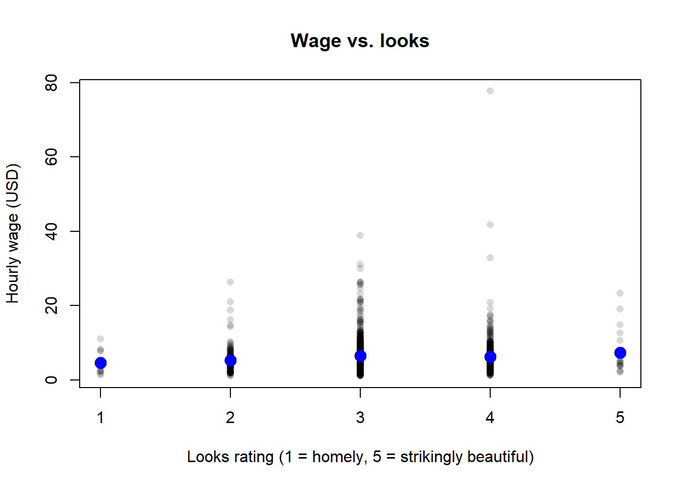
The `beauty` dataset, used by Hammermesh and Biddle (1994) and reproduced in @wooldridge2020, contains hourly wages and a five-point rating of physical appearance for a sample of U.S. workers. The variable `looks` takes integer values from 1 ("homely") to 5 ("strikingly beautiful"), with 3 being "average". The variable `wage` is the hourly wage in U.S. dollars.
We start with summary statistics and a frequency table of `looks`.
```{r ch02-beauty-summary}
summary(beauty$wage)
summary(beauty$looks)
table(beauty$looks)
```
Most workers are rated 3 ("average") --- the marginal categories 1 and 5 are sparse. This already tells us that the slope of a regression of wage on looks will be driven almost entirely by the contrast among categories 2, 3, and 4.
Before any regression, let us compute the mean wage in each looks category. This is the *non-parametric* conditional mean and gives us a benchmark against which to compare the OLS fit.
```{r ch02-beauty-condmean}
tapply(beauty$wage, beauty$looks, mean)
```
Mean wages rise (modestly and not entirely monotonically) with looks. The natural single-number summary of this pattern is the slope of the OLS line.
A scatter plot of the raw data, with the conditional means superimposed, makes the story visible.
```{r ch02-beauty-scatter}
#| fig-cap: "Hourly wage vs. looks rating in the beauty dataset. Blue dots are conditional means by looks category."
cm <- tapply(beauty$wage, beauty$looks, mean)
plot(beauty$looks, beauty$wage,
     xlab = "Looks rating (1 = homely, 5 = strikingly beautiful)",
     ylab = "Hourly wage (USD)",
     main = "Wage vs. looks",
     pch = 16, col = rgb(0, 0, 0, 0.15))
points(as.numeric(names(cm)), cm, pch = 19, col = "blue", cex = 1.6)
```
Now we estimate the simple linear regression of wage on looks with `lm()`:
```{r ch02-beauty-lm}
fit_beauty <- lm(wage ~ looks, data = beauty)
summary(fit_beauty)
```
::: {.callout-note}
## Reading the `summary()` output, column by column
Every column of R's `lm()` summary maps to a quantity we have already named in this chapter (or will name in Chapter 4). Use this once as a Rosetta stone --- the columns recur in every regression `summary()` you will ever read.
- `Estimate` → the OLS coefficient $\hat\beta_j$ (intercept $\hat\beta_0$ in the first row, slope $\hat\beta_1$ in the second), defined in §2.4.3.
- `Std. Error` → the standard error $\operatorname{se}(\hat\beta_j) = \hat\sigma / \sqrt{\mathrm{SST}_x}$ from §2.9.
- `t value` → the ratio $\hat\beta_j / \operatorname{se}(\hat\beta_j)$. We treat it formally in Chapter 4 §4.3; for now, read it as "how many standard errors is the estimate away from zero."
- `Pr(>|t|)` → the two-sided $p$-value for $H_0: \beta_j = 0$. We treat it formally in Chapter 4 §4.7.
- `Residual standard error` → $\hat\sigma$ from §2.9, i.e. the square root of $\hat\sigma^2 = \mathrm{SSR}/(n - 2)$.
- `Multiple R-squared` → the $R^2$ from §2.10 --- the fraction of the variation in `wage` explained by `looks`.
- The bottom-line `F-statistic` tests $H_0: \beta_1 = 0$ in this single-regressor setting; in Chapter 4 we generalise it to joint hypotheses on several coefficients.
:::
Reading the output:
- The estimated intercept $\hat\beta_0$ is the predicted wage for a worker with `looks = 0` --- a value outside the range of the data, so the intercept has no direct economic interpretation here.
- The estimated slope $\hat\beta_1$ on `looks` is the change in predicted hourly wage for a one-point increase in the looks rating. A worker rated 4 ("above average") is predicted to earn about $\hat\beta_1$ dollars per hour more than a worker rated 3 ("average"), on average.
- The standard error of $\hat\beta_1$, the $t$-statistic and the $p$-value tell us whether the slope is statistically distinguishable from zero. We treat these formally in Chapter 4; for now, note that the slope is significantly different from zero at conventional levels.
- The **Residual standard error** at the bottom of `summary()` is $\hat\sigma$ from §2.9.
- The **Multiple R-squared** is the $R^2$ from §2.10. It is small (1--2 %): looks alone explains only a tiny share of the variation in wages. That does not invalidate the slope --- it simply reminds us that wages depend on far more than looks (education, experience, occupation, …), most of which we will add as controls in Chapter 3.
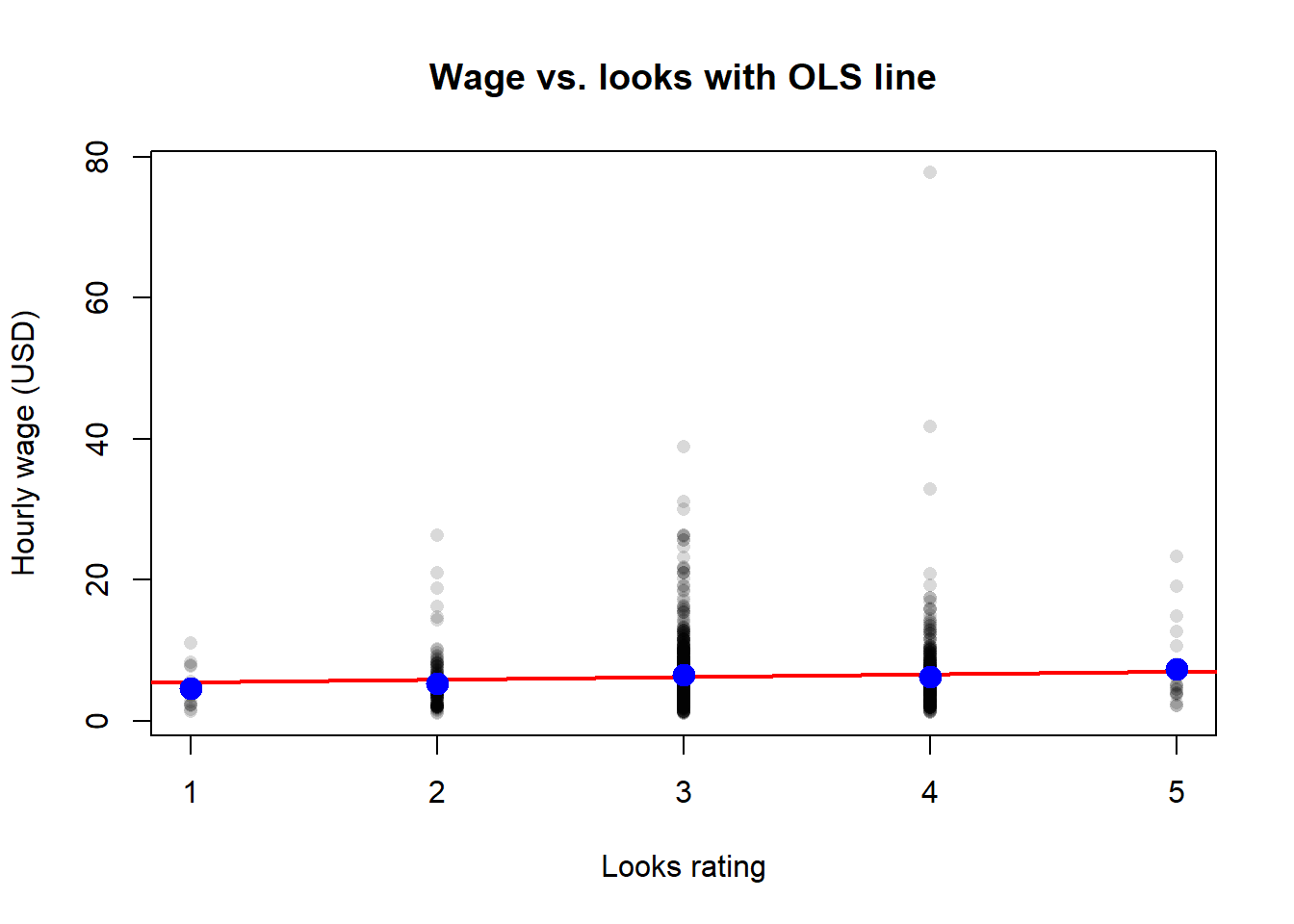
To finish, overlay the OLS line on the scatter:
```{r ch02-beauty-fitline}
#| fig-cap: "OLS line and conditional means for the wage--looks regression."
plot(beauty$looks, beauty$wage,
     xlab = "Looks rating", ylab = "Hourly wage (USD)",
     main = "Wage vs. looks with OLS line",
     pch = 16, col = rgb(0, 0, 0, 0.15))
abline(fit_beauty, col = "red", lwd = 2)
points(as.numeric(names(cm)), cm, pch = 19, col = "blue", cex = 1.6)
```
The red OLS line approximates the trend in the blue conditional means but does not interpolate them exactly --- a linear model is an approximation.
A useful sanity check is to verify the decomposition $\mathrm{SST} = \mathrm{SSE} + \mathrm{SSR}$ and the identity $R^2 = 1 - \mathrm{SSR}/\mathrm{SST}$ from §2.10:
```{r ch02-beauty-r2}
yhat <- fitted(fit_beauty)
uhat <- resid(fit_beauty)
y    <- beauty$wage
SST  <- sum((y - mean(y))^2)
SSE  <- sum((yhat - mean(y))^2)
SSR  <- sum(uhat^2)
c(SST = SST, SSE_plus_SSR = SSE + SSR)
c(R2_manual = 1 - SSR / SST, R2_lm = summary(fit_beauty)$r.squared)
```
The two pairs of numbers match (up to numerical rounding), as the theory predicts.
### Lab B --- Birth weight and smoking (`bwght`)
The `bwght` dataset records the birth weight (in ounces) and average daily cigarette consumption of the mother during pregnancy, among other variables, for a sample of U.S. births. Maternal smoking is one of the most studied determinants of birth weight, with clear medical plausibility for a *negative* effect.
```{r ch02-bwght-summary}
summary(bwght$bwght)
summary(bwght$cigs)
mean(bwght$cigs)
```
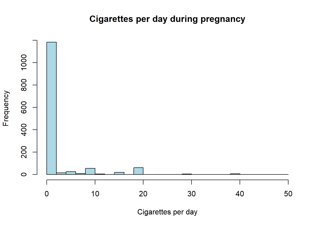
Most mothers in the sample do not smoke (the median of `cigs` is zero). Among those who do, daily consumption can be as high as 50 cigarettes. The histogram makes the heavy right tail obvious:
```{r ch02-bwght-hist}
#| fig-cap: "Distribution of cigarettes smoked per day during pregnancy (bwght)."
hist(bwght$cigs,
     main  = "Cigarettes per day during pregnancy",
     xlab  = "Cigarettes per day",
     col   = "lightblue",
     breaks = 20)
```
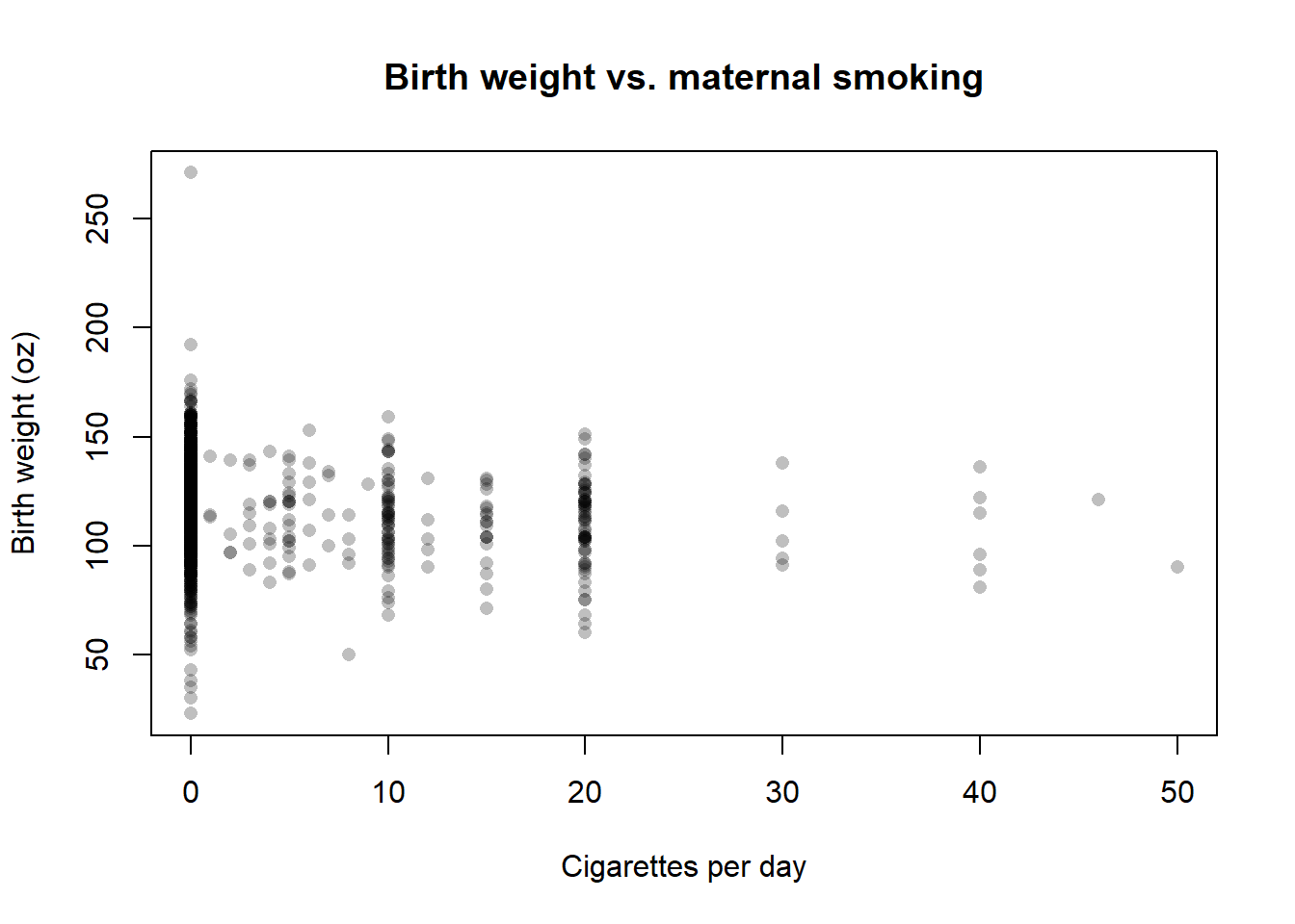
A scatter of birth weight against cigarettes:
```{r ch02-bwght-scatter}
#| fig-cap: "Birth weight in ounces vs. cigarettes per day."
plot(bwght$cigs, bwght$bwght,
     xlab = "Cigarettes per day",
     ylab = "Birth weight (oz)",
     main = "Birth weight vs. maternal smoking",
     pch  = 16, col = rgb(0, 0, 0, 0.25))
```
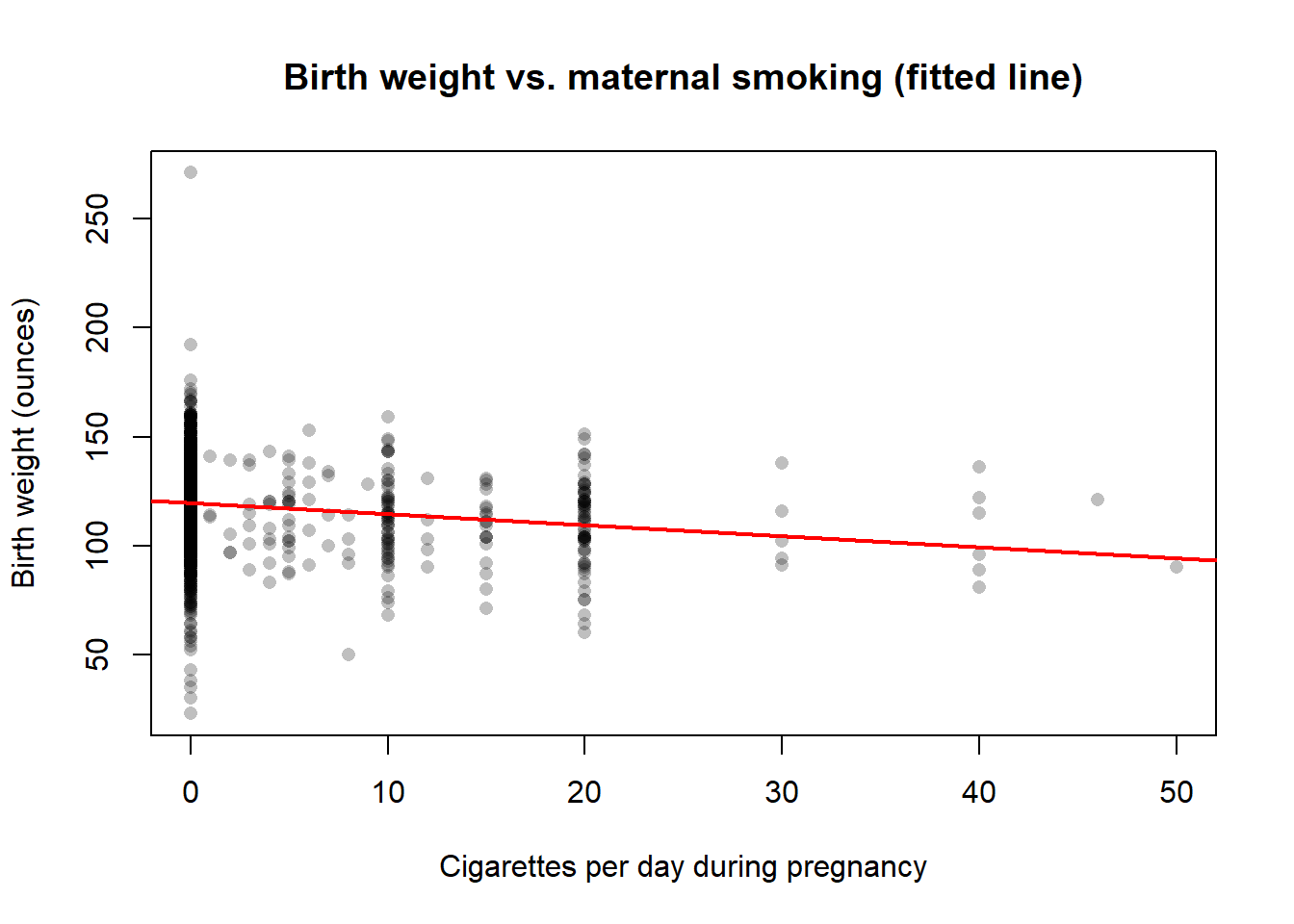
Now the simple linear regression of `bwght` on `cigs`:
```{r ch02-bwght-lm}
fit_bwght <- lm(bwght ~ cigs, data = bwght)
summary(fit_bwght)
plot(bwght$cigs, bwght$bwght,
     xlab = "Cigarettes per day during pregnancy",
     ylab = "Birth weight (ounces)",
     main = "Birth weight vs. maternal smoking (fitted line)",
     pch  = 16, col = rgb(0, 0, 0, 0.25))
abline(fit_bwght, col = "red", lwd = 2)
```
Interpretation:
- $\hat\beta_0$ is the predicted birth weight for a baby whose mother does *not* smoke during pregnancy (`cigs = 0`). Unlike the beauty regression, this is a meaningful value because the median of `cigs` is zero.
- $\hat\beta_1$ is the change in predicted birth weight for one extra cigarette per day. The estimated slope is approximately $-0.51$ ounces per cigarette, so smoking ten more cigarettes per day is associated with roughly $10 \times (-0.51) \approx -5.1$ ounces of birth weight. The negative sign is consistent with everything we know from medicine.
- The $R^2$ is again small. Birth weight depends on dozens of factors --- maternal nutrition, age, prior births, prenatal care --- and `cigs` is only one of them. As in Lab A, a small $R^2$ does not invalidate the slope estimate.
Whether the estimated $-0.51$ is the *causal* effect of smoking on birth weight is a different question. If mothers who smoke also differ from non-smokers in income, education, and nutrition, and if those characteristics independently affect birth weight, then SLR.4 fails and $\hat\beta_1$ is biased. We will revisit this exact dataset in Chapter 3 once we have the multiple regression tools needed to address it.
## Self-check {.unnumbered}
Seven short multiple-choice questions. Try each one before opening the answer.
::: {.callout-tip collapse="true"}
## Q1. The slope $\beta_1$
In the simple regression model $y = \beta_0 + \beta_1 x + u$, the slope $\beta_1$ measures:
- A. The correlation between $x$ and $y$.
- B. The expected change in $y$ when $x$ increases by one unit, holding all factors in $u$ fixed.
- C. The expected value of $y$ when $x = 0$.
- D. The variance of $y$ explained by $x$.
**Answer: B.** $\beta_1$ is the *ceteris paribus* change in the conditional mean of $y$. C describes the intercept $\beta_0$; A is the correlation (a different, scale-free quantity); D is $R^2$.
:::
::: {.callout-tip collapse="true"}
## Q2. The zero-conditional-mean assumption
The assumption $\mathbb{E}[u \mid x] = 0$ implies:
- A. The error $u$ is normally distributed.
- B. $\operatorname{Var}(u \mid x)$ is constant in $x$.
- C. $\mathbb{E}[u] = 0$ and $\operatorname{Cov}(x, u) = 0$.
- D. $x$ is measured without error.
**Answer: C.** Zero conditional mean implies both an unconditional mean of zero (by iterated expectations) and zero covariance between $x$ and $u$. B is the separate homoskedasticity assumption SLR.5; A and D are unrelated.
:::
::: {.callout-tip collapse="true"}
## Q3. The OLS slope formula
The OLS estimator of $\beta_1$ in the simple regression $y = \beta_0 + \beta_1 x + u$ can be written as:
- A. $\hat\beta_1 = \bar y / \bar x$.
- B. $\hat\beta_1 = \widehat{\operatorname{Var}}(y) / \widehat{\operatorname{Cov}}(x, y)$.
- C. $\hat\beta_1 = \widehat{\operatorname{Cov}}(x, y) / \widehat{\operatorname{Var}}(x)$.
- D. $\hat\beta_1 = \bar y - \hat\beta_0 \bar x$.
**Answer: C.** The slope is the sample covariance of $x$ and $y$ over the sample variance of $x$. D is (a rearranged) formula for the intercept; A and B are not OLS estimators.
:::
::: {.callout-tip collapse="true"}
## Q4. Mechanical properties of OLS residuals
Which of the following is **NOT** an algebraic property of OLS residuals $\hat u_i$?
- A. $\sum_i \hat u_i = 0$.
- B. $\sum_i x_i \hat u_i = 0$.
- C. The OLS line passes through $(\bar x, \bar y)$.
- D. $\hat u_i$ are uncorrelated with the unobserved error $u_i$.
**Answer: D.** A, B, and C follow directly from the first-order conditions and hold in every sample. D is a statement about the population disturbance $u_i$, which is never observable; there is no algebraic identity relating $\hat u_i$ to $u_i$.
:::
::: {.callout-tip collapse="true"}
## Q5. Unbiasedness vs. BLUE
Under SLR.1--SLR.4 only (no homoskedasticity), OLS is:
- A. Unbiased: $\mathbb{E}[\hat\beta_j] = \beta_j$.
- B. The Best Linear Unbiased Estimator (BLUE).
- C. Consistent but biased.
- D. Normally distributed.
**Answer: A.** Unbiasedness needs only SLR.1--SLR.4. Adding SLR.5 (homoskedasticity) is what upgrades OLS to BLUE via the Gauss--Markov theorem.
:::
::: {.callout-tip collapse="true"}
## Q6. Precision of $\hat\beta_1$
Which of the following increases the precision of $\hat\beta_1$ (smaller sampling variance)?
- A. A larger error variance $\sigma^2$.
- B. A smaller sample size.
- C. Less variation in $x$.
- D. More variation in $x$ (larger $\mathrm{SST}_x$).
**Answer: D.** The variance formula is $\operatorname{Var}(\hat\beta_1 \mid \mathbf{x}) = \sigma^2 / \mathrm{SST}_x$. Larger $\mathrm{SST}_x$ shrinks the variance. A and B do the opposite; C is a re-statement of "less precision".
:::
::: {.callout-tip collapse="true"}
## Q7. What $R^2$ does and does not tell us
A low $R^2$ in a simple linear regression means:
- A. OLS is biased.
- B. $x$ has no causal effect on $y$.
- C. $x$ explains a small share of the variation in $y$, but $\hat\beta_1$ can still be unbiased and policy-relevant.
- D. The Gauss--Markov assumptions are violated.
**Answer: C.** $R^2$ is a measure of fit, not of bias or causality. A small $R^2$ is fully compatible with an unbiased and economically meaningful slope, as the wage--looks and birth-weight--smoking labs illustrate.
:::
## Exercises {.unnumbered}
**Exercise 2.1 ★ --- Reading a fitted equation.** A regression on 1{,}000 workers gives the fitted line $\widehat{\text{Wage}} = 800 + 15 \times \text{Education}$, where wage is in euros per month and education is in years.
(a) Interpret $\hat\beta_0$ and $\hat\beta_1$ in words.
(b) What is the predicted wage of a worker with 12 years of schooling?
(c) Two workers differ by 4 years of schooling. By how much do their predicted wages differ?
(d) Why should you be wary of the prediction at `educ = 0`?
::: {.callout-tip collapse="true"}
## Show answer
(a) $\hat\beta_0 = 800$ is the predicted wage at `educ = 0` (800 €/month). $\hat\beta_1 = 15$ is the predicted increase in monthly wage per extra year of schooling.
(b) $800 + 15 \times 12 = 980$ €/month.
(c) $4 \times 15 = 60$ €/month.
(d) Because `educ = 0` is far below the lowest value in any realistic schooling sample --- the prediction is an extrapolation and may be unreliable.
:::
**Exercise 2.2 ★ --- Algebra of OLS, by hand.** Consider the toy data $x = (1, 2, 3, 4, 5)$ and $y = (3, 4, 2, 5, 6)$.
(a) Compute $\bar x$ and $\bar y$.
(b) Compute $\hat\beta_1$ using the formula in §2.4.3.
(c) Compute $\hat\beta_0$.
(d) Verify your answer in R against `coef(lm(y ~ x))`.
::: {.callout-tip collapse="true"}
## Show answer
(a) $\bar x = 3$, $\bar y = 4$.
(b) Numerator: $\sum (x_i - \bar x)(y_i - \bar y) = (-2)(-1) + (-1)(0) + 0(-2) + 1(1) + 2(2) = 2 + 0 + 0 + 1 + 4 = 7$. Denominator: $\sum (x_i - \bar x)^2 = 4 + 1 + 0 + 1 + 4 = 10$. So $\hat\beta_1 = 7/10 = 0.7$.
(c) $\hat\beta_0 = \bar y - \hat\beta_1 \bar x = 4 - 0.7 \times 3 = 1.9$.
(d) In R: `coef(lm(c(3,4,2,5,6) ~ c(1,2,3,4,5)))` returns the same numbers.
:::
**Exercise 2.3 ★ --- Variance of the OLS slope.** State, in one sentence each, how the variance $\operatorname{Var}(\hat\beta_1)$ changes if:
(a) the sample size $n$ doubles (holding the distribution of $x$ fixed);
(b) the error variance $\sigma^2$ doubles;
(c) the regressor $x$ is rescaled from minutes to hours (divided by 60).
::: {.callout-tip collapse="true"}
## Show answer
(a) $\mathrm{SST}_x$ roughly doubles, so the variance is approximately halved. (b) The variance doubles (it is linear in $\sigma^2$). (c) The variance of the *slope on the rescaled regressor* increases by a factor of $60^2 = 3600$: scaling $x$ by $c$ multiplies $\hat\beta_1$ by $1/c$, so its variance is multiplied by $1/c^2$.
:::
**Exercise 2.4 ★★ --- Change of units.** Show that if we redefine the regressor as $x^* = c \cdot x$ (for some constant $c \neq 0$) without changing $y$, the new OLS estimators are $\hat\beta_1^* = \hat\beta_1 / c$ and $\hat\beta_0^* = \hat\beta_0$. Verify your derivation empirically on `sleep75`: regress `sleep` on `totwrk` (minutes per week) and then on `totwrk/60` (hours per week), and confirm that the intercept is unchanged while the slope scales by $60$.
*A full answer is given in the Instructor Edition.*
**Exercise 2.5 ★★ --- Unbiasedness by simulation.** Simulate $1{,}000$ samples of size $n = 200$ from $y = 1 + 2x + u$ with $x \sim N(0, 1)$ and $u \sim N(0, 1)$. Compute $\hat\beta_1$ in each sample and show that its mean across replications is close to 2, while the standard deviation across replications is close to the theoretical $\sigma / \sqrt{\mathrm{SST}_x}$ for a typical draw. Plot the histogram of $\hat\beta_1$.
*A full answer is given in the Instructor Edition.*
**Exercise 2.6 ★★★ --- Why dropping the intercept biases the slope.** Suppose the true model is $y = \beta_0 + \beta_1 x + u$ with $\beta_0 \neq 0$ and $\mathbb{E}[u \mid x] = 0$, but the researcher *imposes* $\beta_0 = 0$ and fits the regression through the origin $\tilde y_i = \tilde\beta_1 x_i$.
(a) Derive the closed-form expression for $\tilde\beta_1 = \sum_i x_i y_i / \sum_i x_i^2$ as the minimiser of $\sum_i (y_i - \tilde\beta_1 x_i)^2$.
(b) Show that $\mathbb{E}[\tilde\beta_1] = \beta_1 + \beta_0 \cdot \mathbb{E}[x] / \mathbb{E}[x^2]$, so $\tilde\beta_1$ is biased whenever $\beta_0 \neq 0$ and $\mathbb{E}[x] \neq 0$.
(c) Under what specific condition on the population is the no-intercept slope nonetheless unbiased?
*A full answer is given in the Instructor Edition.*