6  Prediction and Model Selection

Status: ported 2026-05-18. Reviewed by editor: pending.

Learning outcomes

By the end of this chapter the reader should be able to:

• Distinguish causal inference from prediction as two different econometric goals, and explain why a model that predicts well is not automatically a good causal model.
• Compute the point prediction \(\hat y_0\) for a new observation with regressor values \(x_0\), both in the simple and multiple linear regression settings.
• Construct and interpret the two distinct interval estimates: the confidence interval for the conditional mean \(\mathbb{E}[y \mid x_0]\), and the prediction interval for an individual outcome \(y_0\).
• Explain why the prediction interval is always wider than the confidence interval for the mean, and identify the conditions under which both intervals are wider.
• Compare nested models using \(R^2\), adjusted \(R^2\), the Akaike (AIC) and Bayesian (BIC) information criteria, and the nested \(F\)-test.
• Use predict(), AIC(), BIC(), and anova() in R to predict from a fitted model and to choose among competing specifications.

Motivating empirical question

Two recruiters interview the same candidate — a 24-year-old with 16 years of education, 5 years of experience, and 2 years of tenure — and both fit the same wage regression to the same data. The first reports a 95% interval of [$5.7, $7.2] for the expected wage; the second reports [$0.5, $12.4]. Both are correct. Which interval is which?

The answer turns on a distinction that is easy to miss: the first recruiter is reporting uncertainty about the average wage of people like this candidate, while the second is reporting uncertainty about this candidate’s actual wage. The same fitted model produces both numbers — they answer different questions. This chapter is about that distinction and the related question of how to choose between competing models in the first place.

6.1 5.1 Causality vs. prediction

Up to Chapter 4 we have used regression for one purpose: to estimate the ceteris paribus effect of \(x\) on \(y\). The coefficient \(\beta_j\) was the object of interest, and the entire apparatus of Gauss–Markov assumptions, \(t\)-tests, and \(F\)-tests was in the service of getting \(\hat\beta_j\) right — unbiased, efficient, and with valid standard errors.

Econometrics also has a second, equally legitimate use: prediction. Here we do not particularly care about the value of any individual \(\beta_j\); we care about the accuracy of the fitted value \(\hat y_0\) for a new observation.

The two goals overlap but are not the same:

• Causal inference. The target is \(\partial \mathbb{E}[y \mid x] / \partial x_j\). The decisive assumption is MLR.4 (zero conditional mean): \(\mathbb{E}[u \mid x_1, \dots, x_k] = 0\). Coefficients are interpreted; the typical statement is “a one-unit increase in \(x_j\) causes an expected change of \(\beta_j\) in \(y\), holding other factors constant”.
• Prediction. The target is \(\hat y_0\) for a new \(x_0\). The decisive assumption is stability: the new \((y_0, x_0)\) is drawn from the same population as the sample. Coefficients need not be interpretable; we want regressors with strong predictive power and high (in-sample and out-of-sample) fit.

A model can be excellent for one purpose and poor for the other. A predictor of road accidents that includes “ice-cream sales” as a regressor may work well because ice cream proxies for hot weather; it is useless for causal policy advice about ice cream. Conversely, an instrumental-variables estimate of the return to schooling might identify a clean causal parameter from a tiny slice of variation in the data, while leaving most of the variability in wages unexplained.

WarningCommon mistake: choosing the model with the highest \(R^2\) and reading off causal effects

A high \(R^2\) tells you that the fitted values track \(y\) well. It does not tell you that any individual coefficient measures a causal effect. The identification strategy — random assignment, an instrument, a natural experiment, or a credible argument that \(\mathbb{E}[u \mid x] = 0\) — is what licences causal interpretation. Fit-based selection criteria such as adjusted \(R^2\), AIC, and BIC are tools for prediction; they cannot rescue a model that suffers from omitted-variable bias.

6.2 5.2 Point prediction

Consider, for clarity, the simple linear regression (SLR) model:

\[ y_i = \beta_0 + \beta_1 x_i + u_i, \qquad \mathbb{E}[u_i \mid x_i] = 0. \]

Given the OLS estimates \((\hat\beta_0, \hat\beta_1)\) and a new value \(x_0\) of the regressor, the point prediction is just the fitted value of the regression at \(x_0\):

\[ \hat y_0 = \hat\beta_0 + \hat\beta_1 x_0. \]

The same construction extends, term by term, to multiple linear regression (MLR). If \(x_0 = (1, x_{01}, x_{02}, \dots, x_{0k})\) is the row vector of regressor values for the new observation, then

\[ \hat y_0 = \hat\beta_0 + \hat\beta_1 x_{01} + \hat\beta_2 x_{02} + \cdots + \hat\beta_k x_{0k}. \]

How good is this prediction? The natural quantity is the forecast error:

\[ f \equiv y_0 - \hat y_0 = (\beta_0 + \beta_1 x_0 + u_0) - (\hat\beta_0 + \hat\beta_1 x_0). \]

Taking the conditional expectation under MLR.1–MLR.4,

\[ \mathbb{E}[f \mid x_0] = (\beta_0 + \beta_1 x_0) - \mathbb{E}[\hat\beta_0 + \hat\beta_1 x_0] = 0. \]

So \(\hat y_0\) is an unbiased predictor of \(y_0\). In fact, under SLR.1–SLR.5 (and their MLR counterparts), one can show that \(\hat y_0\) has the smallest variance among all linear unbiased predictors: it is the Best Linear Unbiased Predictor (BLUP).

Warning\(\hat y_0\) plays a dual role

The same number \(\hat y_0\) is both the point prediction of the individual outcome \(y_0\) and the estimate of the conditional mean \(\mathbb{E}[y \mid x_0]\). The two interpretations of \(\hat y_0\) are numerically identical, but they have different uncertainty. The next section makes this concrete.

6.3 5.3 Forecast variance and prediction intervals

A point estimate is rarely enough. We need an interval that quantifies uncertainty — and there are two distinct uncertainties to quantify.

6.3.1 5.3.1 Confidence interval for the conditional mean \(\mathbb{E}[y \mid x_0]\)

The conditional mean \(\mathbb{E}[y \mid x_0] = \beta_0 + \beta_1 x_0\) is a fixed (non-random) population quantity. Its estimator is \(\hat y_0 = \hat\beta_0 + \hat\beta_1 x_0\), which is random because the OLS estimates are random. Its variance is

\[ \operatorname{Var}(\hat y_0 \mid x) = \sigma^2 \left[\frac{1}{n} + \frac{(x_0 - \bar x)^2}{\mathrm{SST}_x}\right], \]

where \(\mathrm{SST}_x = \sum_{i=1}^{n} (x_i - \bar x)^2\) is the total sum of squares of the regressor. Replacing \(\sigma^2\) by the estimator \(\hat\sigma^2 = \mathrm{SSR}/(n - k - 1)\), the \(100(1 - \alpha)\%\) confidence interval for the mean prediction is

\[ \hat y_0 \;\pm\; t_c \cdot \hat\sigma \sqrt{\frac{1}{n} + \frac{(x_0 - \bar x)^2}{\mathrm{SST}_x}}, \]

with \(t_c\) the appropriate critical value of a \(t\)-distribution with \(n - k - 1\) degrees of freedom.

6.3.2 5.3.2 Prediction interval for an individual outcome \(y_0\)

The new outcome \(y_0 = \beta_0 + \beta_1 x_0 + u_0\) is random because both the OLS estimates and the new error \(u_0\) are random. Assuming \(u_0\) is independent of the sample,

\[ \operatorname{Var}(y_0 - \hat y_0 \mid x) = \sigma^2 \left[1 + \frac{1}{n} + \frac{(x_0 - \bar x)^2}{\mathrm{SST}_x}\right]. \]

The extra “\(1\)” inside the brackets is the contribution of \(u_0\) — the irreducible part of the new draw that no amount of data could ever predict. The \(100(1 - \alpha)\%\) prediction interval for \(y_0\) is

\[ \hat y_0 \;\pm\; t_c \cdot \hat\sigma \sqrt{1 + \frac{1}{n} + \frac{(x_0 - \bar x)^2}{\mathrm{SST}_x}}. \]

In MLR the same logic gives \(\operatorname{Var}(y_0 - \hat y_0 \mid X) = \sigma^2 [1 + x_0'(X'X)^{-1} x_0]\), with the CI for the mean obtained by dropping the “\(1\)” in the brackets.

NoteThe two intervals at a glance

Quantity targeted	Variance ingredient	Interval	Width
Mean \(\mathbb{E}[y \mid x_0]\)	\(1/n + (x_0 - \bar x)^2 / \mathrm{SST}_x\)	Confidence interval	Narrower
Individual \(y_0\)	\(1 + 1/n + (x_0 - \bar x)^2 / \mathrm{SST}_x\)	Prediction interval	Wider

The PI is always wider than the CI. The gap is governed by the “1”: the irreducible variance of the new draw \(u_0\).

A few more observations on the formulas:

• Both variances shrink as \(n\) grows — with infinite data the CI for the mean would collapse to a point, but the PI would not, because the “1” never goes away.
• Both variances grow as \(x_0\) moves away from the sample mean \(\bar x\). Predictions are most precise near the centre of the data; predicting at the edges (or extrapolating beyond them) is dangerous.
• Both variances shrink as \(\mathrm{SST}_x\) grows. More spread-out regressors give more leverage to pin down the slope, which in turn tightens prediction.

6.3.3 5.3.3 Worked numerical example

Suppose we have estimated the SLR

\[ \hat y = 2.0 + 0.7\,x, \]

with sample size \(n = 100\), \(\bar x = 12\), \(\mathrm{SST}_x = 200\), and \(\hat\sigma^2 = 4\) (so \(\hat\sigma = 2\)). We want to predict at \(x_0 = 16\). Using \(t_c \approx 1.98\) for a 95% interval with 98 degrees of freedom:

• Point prediction. \(\hat y_0 = 2.0 + 0.7 \times 16 = 13.2\).

• CI for the mean \(\mathbb{E}[y \mid x_0]\). \[ \mathrm{se}(\hat y_0) = \hat\sigma \sqrt{\tfrac{1}{100} + \tfrac{(16-12)^2}{200}} = 2\sqrt{0.01 + 0.08} = 0.6. \] \[ \text{95\% CI:} \quad 13.2 \pm 1.98 \times 0.6 = [12.01,\ 14.39]. \]

• Prediction interval for \(y_0\). \[ \mathrm{se}(f) = \hat\sigma \sqrt{1 + \tfrac{1}{100} + \tfrac{(16-12)^2}{200}} = 2\sqrt{1.09} \approx 2.088. \] \[ \text{95\% PI:} \quad 13.2 \pm 1.98 \times 2.088 = [9.06,\ 17.34]. \]

The CI is roughly \(\pm 1.20\) wide around the point prediction; the PI is roughly \(\pm 4.14\) wide. The ratio is set by the relative size of the “\(1\)” against \(1/n + (x_0 - \bar x)^2/\mathrm{SST}_x = 0.09\). Here the new-draw uncertainty dwarfs the parameter uncertainty by an order of magnitude.

6.4 5.4 Prediction in MLR

Real wage models include more than one regressor. Nothing essential changes in the construction of \(\hat y_0\) and the two intervals — the formulas just become vector–matrix versions of the SLR formulas.

For a row vector \(x_0 = (1, x_{01}, \dots, x_{0k})\),

\[ \hat y_0 = x_0' \hat\beta, \qquad \operatorname{Var}(y_0 - \hat y_0 \mid X) = \sigma^2 \left[1 + x_0' (X'X)^{-1} x_0 \right]. \]

Dropping the “\(1\)” gives the variance of \(\hat y_0\) as an estimator of \(\mathbb{E}[y \mid x_0]\). In R, the function predict() does all of this automatically with interval = "confidence" or interval = "prediction". The user supplies the new \(x_0\) as a data frame; the function returns the fit and the bounds. We try this on wage1 in the lab.

WarningDon’t extrapolate

The prediction formulas assume that \((y_0, x_0)\) comes from the same population as the sample. If \(x_0\) is far outside the range of the regressors actually observed — predicting wages for someone with 30 years of education and 80 years of experience, say — both intervals can be technically computed, but neither is trustworthy. There is no information in the sample about what happens at those values. Stay inside the support of the data.

6.5 5.5 Model selection: \(R^2\), adjusted \(R^2\), AIC, BIC

Suppose we have several candidate regression models for the same outcome. How do we choose? Four criteria are commonly used.

6.5.1 5.5.1 \(R^2\) and the garbage-variable problem

The coefficient of determination

\[ R^2 = \frac{\mathrm{SSE}}{\mathrm{SST}} = 1 - \frac{\mathrm{SSR}}{\mathrm{SST}} \]

measures the proportion of the variation of \(y\) explained by the model. It has one fatal flaw as a model-selection device: adding any regressor cannot reduce \(R^2\). Even a pure noise regressor will, almost surely, slightly increase \(R^2\), because OLS can always find a tiny linear combination of the noise that fits some residual variation by chance.

If we picked our model by maximising \(R^2\), we would include every regressor we could lay our hands on — including dozens of irrelevant ones. The model would fit the sample beautifully and predict horribly out of sample. This is the classic overfitting problem. The slides illustrate it by simulating a model with two genuine regressors \(X_1, X_2\) and then adding 196 “garbage” variables of pure noise: \(R^2\) climbs steadily towards 1 as garbage piles up, even though none of the new variables has any predictive content.

6.5.2 5.5.2 Adjusted \(R^2\)

A simple fix is to penalise complexity. The adjusted \(R^2\) is

\[ \bar R^2 = 1 - \frac{\mathrm{SSR} / (n - k - 1)}{\mathrm{SST} / (n - 1)}, \]

where \(k\) is the number of regressors (excluding the intercept). The numerator \(\mathrm{SSR}/(n - k - 1)\) is \(\hat\sigma^2\), the unbiased estimator of the error variance. Adding a regressor reduces \(\mathrm{SSR}\) but also reduces \(n - k - 1\); \(\bar R^2\) goes up only if the gain in fit beats the cost of the extra parameter.

A few useful facts:

• \(\bar R^2 \le R^2\) always, with equality only when \(k = 0\).
• Unlike \(R^2\), \(\bar R^2\) can decrease when an irrelevant regressor is added — and in the garbage simulation, it does.
• \(\bar R^2\) can in principle be negative if the model is so poor that \(\hat\sigma^2\) exceeds the sample variance of \(y\).

6.5.3 5.5.3 AIC and BIC

The Akaike Information Criterion and the Bayesian Information Criterion combine model fit (a log-likelihood) with a complexity penalty:

\[ \mathrm{AIC} = -2 \ln \hat L + 2(k + 1), \qquad \mathrm{BIC} = -2 \ln \hat L + (k + 1) \ln n. \]

For a linear model with normally distributed errors the log-likelihood is a monotone transformation of \(-\mathrm{SSR}/n\), so up to additive constants

\[ \mathrm{AIC} \approx n \ln\!\left(\frac{\mathrm{SSR}}{n}\right) + 2(k+1), \qquad \mathrm{BIC} \approx n \ln\!\left(\frac{\mathrm{SSR}}{n}\right) + (k+1) \ln n. \]

Lower AIC and BIC indicate better models. Both criteria balance fit (the SSR term) against complexity (the second term). The only difference is the size of the penalty: AIC charges \(2\) per extra parameter, BIC charges \(\ln n\). For \(n \ge 8\), \(\ln n > 2\), so BIC penalises complexity more strongly and tends to select more parsimonious models. AIC is built to minimise prediction error; BIC is built to identify the “true” model when one exists.

WarningAIC and BIC require the same dataset and the same dependent variable

If two models use different dependent variables (e.g. wage and log(wage)), or are estimated on different sub-samples, their AIC and BIC are not comparable — the log-likelihoods are on different scales. The same warning applies to \(R^2\) and \(\bar R^2\).

6.5.4 5.5.4 Nested \(F\)-test

When one model is nested inside another — the smaller model is obtained by setting some coefficients of the larger model to zero — the \(F\)-test of joint restrictions (Chapter 4) is the formal test of “are these extra regressors jointly informative?”. In R, anova(small, big) does it. The test answers a different question from AIC/BIC: it asks whether the data reject the smaller model in favour of the larger, not which model is “best” by some predictive criterion.

6.5.5 5.5.5 Putting it together

In practice we report all four criteria side by side. They usually agree on the broad ranking; when they disagree, the disagreement is informative:

• If \(R^2\) rises but \(\bar R^2\), AIC, and BIC all worsen, the new regressors are noise.
• If \(\bar R^2\) and AIC favour the larger model but BIC favours the smaller, the extra regressors are weakly predictive; with a large sample BIC may be over-penalising. In a purely predictive exercise, lean towards AIC; for parsimony or for picking a “true” model, lean towards BIC.

And, always: model selection criteria choose the model that fits best on the criterion at hand. They do not choose the model that identifies a causal parameter best. That choice belongs to the identification strategy.

6.6 5.6 Lab: Prediction and Model Selection in R

We work with the wage1 dataset of 526 U.S. workers (Chapter 1). The goal is to (i) fit a sequence of nested wage models, (ii) compare them using \(\bar R^2\), AIC, BIC, and an \(F\)-test, (iii) produce point predictions and the two interval estimates for a specific worker, and (iv) visualise the difference between the confidence band for the mean and the prediction band for an individual.

library(wooldridge)
data("wage1")

6.6.1 Step 1 — Fit four nested wage models

We progressively enrich the specification.

model1 <- lm(wage ~ educ, data = wage1)
model2 <- lm(wage ~ educ + exper, data = wage1)
model3 <- lm(wage ~ educ + exper + tenure, data = wage1)
model4 <- lm(wage ~ educ + exper + tenure + female + married, data = wage1)

6.6.2 Step 2 — Compare the four models

Collect \(R^2\), \(\bar R^2\), AIC, and BIC in a single table.

tab <- sapply(list(m1 = model1, m2 = model2, m3 = model3, m4 = model4),
              function(m) c(
                R2    = summary(m)$r.squared,
                AdjR2 = summary(m)$adj.r.squared,
                AIC   = AIC(m),
                BIC   = BIC(m)))
round(tab, 3)

            m1       m2       m3       m4
R2       0.165    0.225    0.306    0.368
AdjR2    0.163    0.222    0.302    0.362
AIC   2777.423 2739.937 2683.662 2638.600
BIC   2790.219 2756.999 2704.988 2668.457

A few things to read off this table:

• \(R^2\) rises monotonically from model1 to model4. That is mechanical: adding regressors cannot decrease \(R^2\).
• \(\bar R^2\) also rises across the four models, indicating that each newly added regressor contributes more fit than its complexity cost.
• AIC and BIC both decrease as we go from model1 to model4 (lower is better). All four criteria agree: of these four specifications, model4 is preferred.

6.6.3 Step 3 — A nested \(F\)-test

Are female and married jointly informative once educ, exper, and tenure are in the model?

anova(model3, model4)

Analysis of Variance Table

Model 1: wage ~ educ + exper + tenure
Model 2: wage ~ educ + exper + tenure + female + married
  Res.Df    RSS Df Sum of Sq      F    Pr(>F)    
1    522 4966.3                                  
2    520 4524.0  2    442.27 25.418 2.938e-11 ***
---
Signif. codes:  0 '***' 0.001 '**' 0.01 '*' 0.05 '.' 0.1 ' ' 1

The \(F\)-statistic compares the two SSRs; if its \(p\)-value is small, we reject the joint null \(H_0:\beta_{\text{female}} = \beta_{\text{married}} = 0\). In wage1 it is very small, confirming the AIC/BIC preference for model4 with a formal test.

6.6.4 Step 4 — The garbage-variable demonstration

Now we deliberately add three pure-noise regressors to model4 and watch what happens to each criterion.

set.seed(42)
wage1$noise1 <- rnorm(nrow(wage1))
wage1$noise2 <- rnorm(nrow(wage1))
wage1$noise3 <- rnorm(nrow(wage1))

model_garbage <- lm(wage ~ educ + exper + tenure + female + married +
                      noise1 + noise2 + noise3, data = wage1)

rbind(
  model4        = c(R2 = summary(model4)$r.squared,
                    AdjR2 = summary(model4)$adj.r.squared,
                    AIC = AIC(model4), BIC = BIC(model4)),
  model_garbage = c(R2 = summary(model_garbage)$r.squared,
                    AdjR2 = summary(model_garbage)$adj.r.squared,
                    AIC = AIC(model_garbage), BIC = BIC(model_garbage)))

                     R2     AdjR2      AIC      BIC
model4        0.3681887 0.3621136 2638.600 2668.457
model_garbage 0.3708921 0.3611573 2642.345 2684.998

Inspect the output: \(R^2\) has risen slightly (as it must), but \(\bar R^2\) has fallen, and both AIC and BIC have increased. The three pure-noise regressors look superficially helpful to plain \(R^2\); every penalised criterion sees through them. This is the entire point of using \(\bar R^2\), AIC, or BIC rather than raw \(R^2\) to choose a model.

6.6.5 Step 5 — Point prediction for a specific worker

Take the candidate from the chapter opening: 16 years of education, 5 years of experience, 2 years of tenure, female, unmarried. We use model4.

new_worker <- data.frame(educ = 16, exper = 5, tenure = 2,
                         female = 1, married = 0)
predict(model4, newdata = new_worker)

      1 
5.90268 

This is \(\hat y_0\) — the recruiter’s single-number wage prediction.

6.6.6 Step 6 — The two intervals

The same predict() function delivers the CI for the mean and the PI for the individual.

predict(model4, newdata = new_worker,
        interval = "confidence", level = 0.95)

      fit      lwr      upr
1 5.90268 5.323082 6.482277

predict(model4, newdata = new_worker,
        interval = "prediction", level = 0.95)

      fit        lwr      upr
1 5.90268 0.07919504 11.72616

The first interval is the recruiter’s answer to “what is the average wage of women with these characteristics?”. The second is the answer to “what wage might this woman actually earn?”. The PI is much wider — in this dataset, an order of magnitude wider — because it includes the irreducible variance of the new draw \(u_0\).

6.6.7 Step 7 — A manual sanity check

To make the formulas concrete, compute the CI by hand and compare:

yhat <- predict(model4, newdata = new_worker, se.fit = TRUE)
tc   <- qt(0.975, df = model4$df.residual)
ci_manual <- c(yhat$fit - tc * yhat$se.fit,
               yhat$fit + tc * yhat$se.fit)
ci_manual

       1        1 
5.323082 6.482277 

# Now the prediction interval, using SE(f)^2 = SE(yhat)^2 + sigma_hat^2
sig2 <- summary(model4)$sigma^2
se_pred <- sqrt(yhat$se.fit^2 + sig2)
pi_manual <- c(yhat$fit - tc * se_pred,
               yhat$fit + tc * se_pred)
pi_manual

          1           1 
 0.07919504 11.72616433 

These should match (to rounding) the bounds returned by predict() in Step 6. The decomposition \(\operatorname{Var}(y_0 - \hat y_0) = \operatorname{Var}(\hat y_0) + \sigma^2\) is the operational version of “two sources of uncertainty: the parameters, and the new draw”.

6.6.8 Step 8 — Visualising CI vs. PI across educ

The two-interval distinction is easiest to see in a picture. We compute both bands across a grid of education values (holding the other regressors fixed) and plot them on top of the fitted line.

grid <- data.frame(educ = seq(0, 20, by = 0.5),
                   exper = 5, tenure = 3,
                   female = 0, married = 1)
ci_band <- predict(model4, newdata = grid, interval = "confidence")
pi_band <- predict(model4, newdata = grid, interval = "prediction")

plot(grid$educ, ci_band[, "fit"], type = "l", lwd = 2, col = "blue",
     xlab = "Years of education",
     ylab = "Predicted wage (USD/hour)",
     main = "CI for the mean vs. PI for an individual",
     ylim = range(pi_band))
lines(grid$educ, ci_band[, "lwr"], lty = 2, col = "blue")
lines(grid$educ, ci_band[, "upr"], lty = 2, col = "blue")
lines(grid$educ, pi_band[, "lwr"], lty = 2, col = "red")
lines(grid$educ, pi_band[, "upr"], lty = 2, col = "red")
legend("topleft",
       legend = c("Fitted", "95% CI (mean)", "95% PI (individual)"),
       col = c("blue", "blue", "red"),
       lty = c(1, 2, 2), lwd = c(2, 1, 1))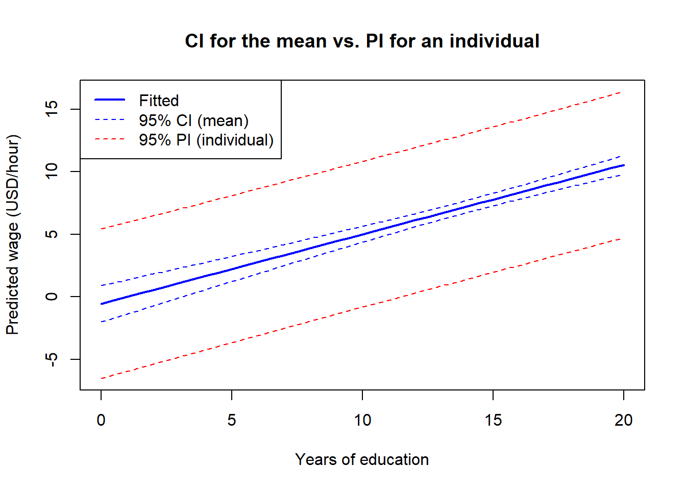

Fitted wage (solid blue) with the 95% confidence band for the conditional mean (dashed blue) and the 95% prediction band for individuals (dashed red), across years of education. Other regressors fixed at exper=5, tenure=3, female=0, married=1.

Two features of the plot are worth pointing out:

• The PI (red) is much wider than the CI (blue) at every value of educ. The vertical gap between the two bands is, essentially, \(\pm t_c \hat\sigma\) — the contribution of \(u_0\).
• Both bands widen at the extremes of educ, away from the sample mean. Predicting wages for a worker with no schooling, or with 20 years of schooling, is intrinsically less precise than predicting near the sample average. This is the \((x_0 - \bar x)^2 / \mathrm{SST}_x\) term in the variance formula doing its work.

We can now answer the opening question. The narrow interval is the CI for the mean wage of workers like the candidate; the wide interval is the PI for this candidate’s wage. Both are produced by the same model, from the same data, with one keystroke of difference in the call to predict().

Self-check

Six short questions. Try each one before opening the answer.

TipQ1. Which interval is which?

A recruiter wants to know the average wage of all workers in the population who share the candidate’s profile. The relevant interval is:

• A. The 95% prediction interval for \(y_0\).
• B. The 95% confidence interval for \(\mathbb{E}[y \mid x_0]\).
• C. The 95% confidence interval for the slope \(\beta_1\).
• D. The OLS residual.

Answer: B. The CI for \(\mathbb{E}[y \mid x_0]\) targets the conditional mean and is the narrower of the two intervals. The PI in option A would be the right choice for “what might this candidate actually earn?”.

TipQ2. Why is the PI wider than the CI?

The 95% prediction interval for \(y_0\) is wider than the 95% confidence interval for \(\mathbb{E}[y \mid x_0]\) because:

• A. The prediction interval uses a larger critical value \(t_c\).
• B. The prediction interval includes the variance of the new error \(u_0\), the irreducible part of the new draw.
• C. The CI ignores the variance of the OLS estimates entirely.
• D. The PI is built with a smaller sample size.

Answer: B. Both intervals use the same \(t_c\). The PI adds a “1” inside the bracket in the variance formula, which captures \(\operatorname{Var}(u_0) = \sigma^2\) — something the data can never predict.

TipQ3. Where are the intervals widest?

Holding the sample fixed, both the CI for the mean and the PI for an individual are widest when:

• A. \(x_0\) equals the sample mean of the regressor.
• B. The sample size is very large.
• C. \(x_0\) is far from the sample mean of the regressor.
• D. The residual variance is zero.

Answer: C. Both variances contain the term \((x_0 - \bar x)^2 / \mathrm{SST}_x\), which grows as \(x_0\) moves away from \(\bar x\). Predictions are most precise near the centre of the data and least precise at the edges; extrapolating beyond the support of the data is dangerous.

TipQ4. Adjusted \(R^2\) and a noise regressor

Adding a pure-noise regressor to an OLS model:

• A. Strictly increases \(R^2\) and strictly increases \(\bar R^2\).
• B. Cannot decrease \(R^2\) but can decrease \(\bar R^2\).
• C. Always lowers \(R^2\) because the new regressor is uninformative.
• D. Has no effect on either criterion.

Answer: B. \(R^2\) never falls when a regressor is added. \(\bar R^2\) penalises complexity through the degrees-of-freedom correction, so an irrelevant regressor can lower it. AIC and BIC will also worsen.

TipQ5. Comparing AIC across models

The Akaike Information Criterion can legitimately be used to compare:

• A. Two models estimated on different sub-samples of the data.
• B. A regression of wage on educ against a regression of log(wage) on educ.
• C. Two models with the same dependent variable, the same data, and different sets of regressors.
• D. Models estimated by different methods (OLS, IV, GMM) on the same data.

Answer: C. AIC (and BIC) are only comparable when the dependent variable, the sample, and the estimation method are the same; otherwise the log-likelihoods are on different scales. The same warning applies to \(R^2\) and \(\bar R^2\).

TipQ6. Causality vs. prediction

The model with the smallest AIC is necessarily the best for:

• A. Both prediction and causal identification of individual coefficients.
• B. Prediction of \(y\) given \(x\) — but not necessarily for identifying the causal effect of a specific regressor.
• C. Causal identification only.
• D. Neither, since AIC is always misleading.

Answer: B. AIC is a predictive criterion. Causal identification depends on the assumption \(\mathbb{E}[u \mid x] = 0\), which is a statement about the design (random assignment, an instrument, a credible argument), not about model fit. A predictively excellent model can still suffer from omitted-variable bias.

Exercises

Exercise 5.1 ★ — The two intervals by hand. Suppose you have fit \(\hat y = 2.0 + 0.7\,x\) on a sample with \(n = 100\), \(\bar x = 12\), \(\mathrm{SST}_x = 200\), and \(\hat\sigma^2 = 4\). Take \(x_0 = 16\) and use \(t_c = 1.98\).

1. Compute the point prediction \(\hat y_0\).
2. Compute the 95% confidence interval for \(\mathbb{E}[y \mid x_0]\).
3. Compute the 95% prediction interval for \(y_0\).
4. Comment briefly on which interval a recruiter would quote and why.

TipShow answer

1. \(\hat y_0 = 2.0 + 0.7 \times 16 = 13.2\).
2. \(\mathrm{se}(\hat y_0) = 2\sqrt{1/100 + 16/200} = 2\sqrt{0.09} = 0.6\), so CI \(= 13.2 \pm 1.98 \times 0.6 = [12.01, 14.39]\).
3. \(\mathrm{se}(f) = 2\sqrt{1 + 0.09} = 2\sqrt{1.09} \approx 2.088\), so PI \(= 13.2 \pm 1.98 \times 2.088 = [9.06, 17.34]\).
4. Both. The CI answers “what is the average wage of workers like the candidate?” — useful for planning aggregate compensation. The PI answers “what might this candidate actually earn?” — useful for an individual job offer. Reporting only one of the two is misleading.

Exercise 5.2 ★ — Reading a selection table. Using wage1, estimate the four nested models from the lab and present a 4-by-4 table of \(R^2\), \(\bar R^2\), AIC, and BIC. Which model wins under each criterion? Do all four criteria agree?

TipShow answer

In wage1 the four criteria agree on the ranking: \(R^2\) and \(\bar R^2\) are highest for model4; AIC and BIC are lowest for model4. Whenever all four agree the choice is easy. When BIC selects a smaller model than AIC (which can happen with larger samples), the gap reflects BIC’s stronger penalty \(\ln n > 2\); the choice then depends on whether you prioritise predictive accuracy (AIC) or parsimony (BIC).

Exercise 5.3 ★ — A 12-year worker and a 20-year worker. Using model4 from the lab, compute the 95% prediction interval for two profiles: (i) educ = 12, exper = 10, tenure = 5, female = 0, married = 1 and (ii) educ = 20, exper = 10, tenure = 5, female = 0, married = 1. Is the second interval wider, narrower, or the same width as the first? Why?

TipShow answer

The second interval is wider. Twenty years of education is far from the sample mean of educ in wage1 (around 12.5 years), so the \((x_0 - \bar x)' (X'X)^{-1} (x_0 - \bar x)\) term in the variance formula is larger. This is the warning against extrapolation: the further \(x_0\) is from the centre of the data, the larger both intervals become, and at some point they become so wide that the prediction is uninformative.

Exercise 5.4 ★★ — A garbage variable in your own data. Take any dataset of your choice (real or simulated). Fit a baseline model with one or two genuine regressors and report \(R^2\), \(\bar R^2\), AIC, BIC. Add five regressors of pure Gaussian noise (rnorm(n)), refit, and report the same four numbers. By how much does each change? Which criterion is fooled, and which is not?

A full answer is given in the Instructor Edition.

Exercise 5.5 ★★ — Causality vs. prediction with a confound. Suppose y is true grade, x is hours studied, and z is innate ability. Hours and ability are positively correlated. You fit two models on a large sample: (a) y ~ x, (b) y ~ x + z. Argue, informally, that:

1. Model (b) has the higher \(R^2\) and higher \(\bar R^2\) — it is the better predictor.
2. Model (a) gives a biased causal estimate of the effect of hours on grades; model (b) does not.
3. AIC and BIC will both prefer model (b).

What conclusion do you draw about using AIC/BIC to choose a causal model?

A full answer is given in the Instructor Edition.

Exercise 5.6 ★★★ — Out-of-sample prediction. Split wage1 into a training set (the first 400 observations) and a test set (the remaining 126). Fit model1 through model4 on the training set. For each model, compute (i) the in-sample \(R^2\) on the training set, and (ii) the out-of-sample mean squared error on the test set: \(\frac{1}{n_{\text{test}}} \sum_{i \in \text{test}} (y_i - \hat y_i)^2\). Which model wins on in-sample \(R^2\)? Which wins on out-of-sample MSE? Comment on the relationship between \(\bar R^2\)/AIC/BIC computed in the training sample and the out-of-sample MSE.

A full answer is given in the Instructor Edition.