3 The Multiple Linear Regression Model
Learning outcomes
By the end of this chapter the reader should be able to:
- Explain why the simple linear regression is rarely enough for credible empirical work, and read each MLR slope as a ceteris paribus (partial) effect.
- Write the multiple linear regression model in matrix form, \(\mathbf{y} = \mathbf{X}\beta + \mathbf{u}\), and derive the OLS solution \(\hat{\beta} = (\mathbf{X}'\mathbf{X})^{-1}\mathbf{X}'\mathbf{y}\).
- State the Gauss–Markov assumptions MLR.1–MLR.5 and recognise which one each empirical pathology violates.
- Show, in matrix form, that OLS is unbiased under MLR.1–MLR.4 and has variance \(\sigma^2(\mathbf{X}'\mathbf{X})^{-1}\) under MLR.1–MLR.5.
- Predict the direction and sign of omitted-variable bias from an auxiliary regression, and verify it numerically on real data.
- Distinguish \(R^2\) from adjusted \(R^2\) and explain when adjusted \(R^2\) may fall as regressors are added.
Motivating empirical question
Once we hold experience, tenure, gender, and marital status constant, what is the return to one additional year of education?
Chapter 1 showed that the raw wage gap by education in wage1 confounds schooling with experience, tenure, and demographics; Chapter 2 fitted a simple regression of wage on educ and explicitly warned that the OLS slope could not be read causally. The multiple linear regression (MLR) model is the workhorse we use to take that warning seriously: by including controls, we move from raw conditional means to partial effects — the change in \(y\) associated with a one-unit change in one regressor, holding all the others fixed.
3.1 Motivation: the problem with simple regression
simple linear regression model \[ y = \beta_0 + \beta_1 x + u \] has one structural weakness: every determinant of \(y\) other than \(x\) is bundled into the error term \(u\). If any of those omitted determinants is correlated with \(x\), then \(\operatorname{Cov}(x,u)\neq 0\), the zero-conditional-mean assumption \(\mathbb{E}[u\mid x]=0\) fails, and OLS is biased for the causal effect of \(x\) on \(y\) (Wooldridge 2020).
NoteExample: education and wages without controls
Suppose \[ \text{wage} = \beta_0 + \beta_1\,\text{educ} + u. \] The error \(u\) contains innate ability, family background, motivation, school quality, and many other unobservables. If more able workers also acquire more education, then \(\operatorname{Cov}(\text{educ}, u) > 0\), and the simple OLS estimator \(\hat\beta_1\) does not isolate the causal return to schooling — it conflates the return to education with the return to whatever drives ability and education together.
The fix is conceptually simple: bring the relevant omitted factors into the model as additional regressors. Replace the simple model by \[ \text{wage} = \beta_0 + \beta_1\,\text{educ} + \beta_2\,\text{exper} + \beta_3\,\text{tenure} + u, \] so that experience and tenure now appear in the systematic part instead of in \(u\). The coefficient \(\beta_1\) in this longer model is interpreted as the change in expected wage for a one-year increase in education, holding experience and tenure fixed. That is the ceteris paribus statement empirical economics aims for.
Two cautions deserve emphasis from the outset:
- Adding controls is not the same as identifying causality. We will see in §3.9 that the bias only disappears for the variables whose relevant confounders we actually include.
- Including too many or highly correlated regressors can inflate variance without removing bias. There is no free lunch.
3.2 The MLR model
NoteDefinition: the multiple linear regression model
With \(k\) regressors \(x_1,\ldots,x_k\), the population MLR model is \[ y = \beta_0 + \beta_1 x_1 + \beta_2 x_2 + \cdots + \beta_k x_k + u. \] Each slope \(\beta_j\) is the partial effect of \(x_j\) on \(y\): \[ \beta_j \;=\; \frac{\partial\, \mathbb{E}[y\mid x_1,\ldots,x_k]}{\partial x_j}. \] That is, \(\beta_j\) measures how the conditional mean of \(y\) shifts when \(x_j\) changes by one unit and all other regressors are held constant.
In the wage example, a fitted equation such as \[ \widehat{\text{wage}} \;=\; 3.0 + 1.5\,\text{educ} + 0.04\,\text{age} + 0.07\,\text{exper} + 0.05\,\text{tenure} \] says: across two workers with the same age, experience, and tenure but differing by one year of schooling, the predicted hourly wage differs by 1.50 dollars on average. The crucial qualifier is the “same age, experience, and tenure” — this is what distinguishes the MLR coefficient from the unconditional regression slope.
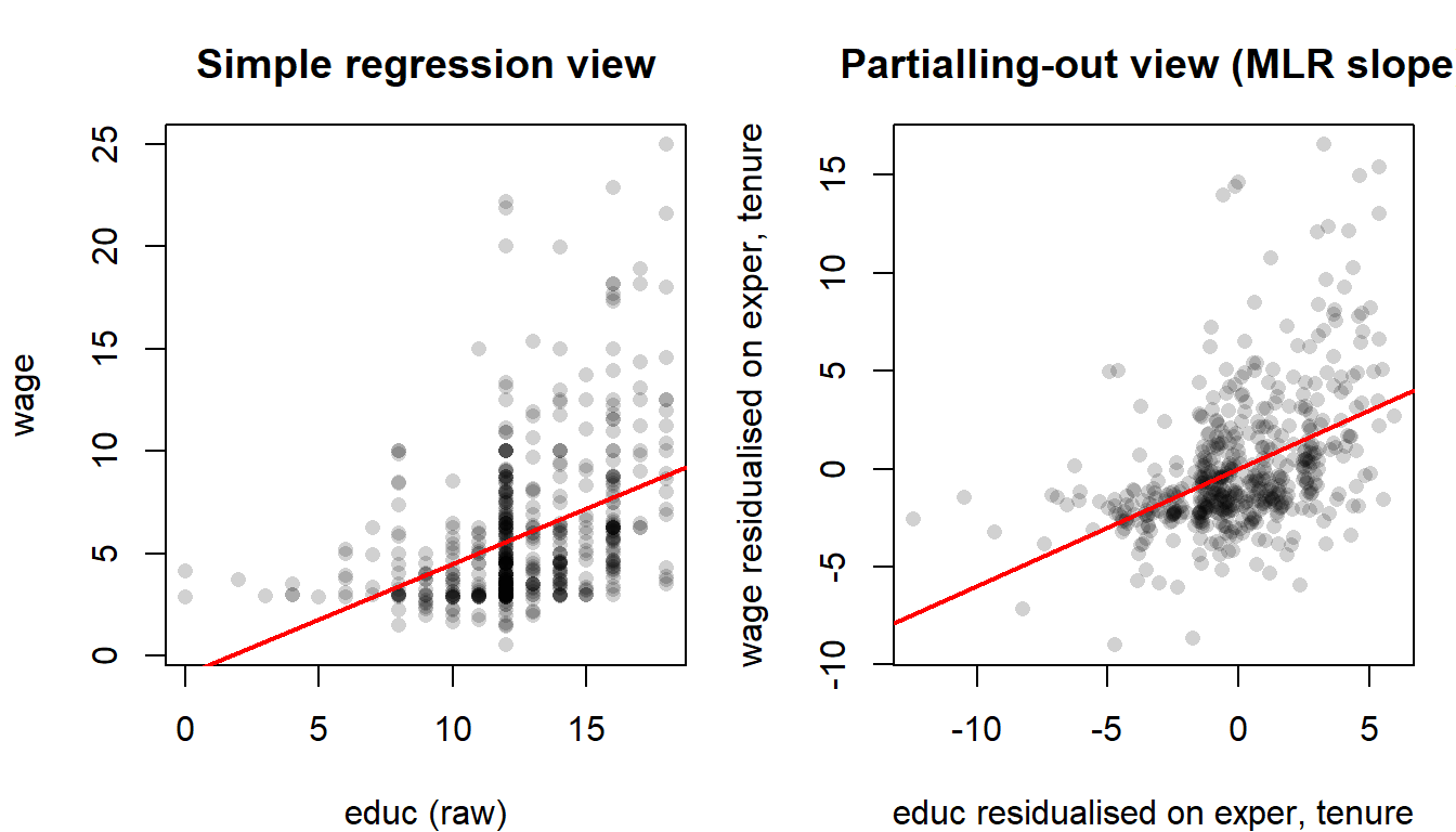
3.3 What does “holding fixed” actually do? Partialling out
A picture before the algebra: what does “holding the other regressors fixed” actually do to the data? The answer is partialling out. To get the MLR slope on educ, first scrub from educ whatever part of it is predictable from exper and tenure (its residualised version), then regress wage — itself residualised on the same controls — on that. The MLR slope on educ is the slope of the resulting scatter.
WarningCommon mistake: forgetting ceteris paribus
A widespread error is to read \(\hat\beta_1\) as “the effect on \(y\) of changing \(x_1\)” without the conditioning clause. In MLR every slope is conditional on the other regressors in the equation. If you change which controls you include, you change what \(\beta_1\) means — not just its numerical value.
3.4 Matrix notation
If matrices and the transpose are rusty, pause here and skim Appendix A.5 (three pages) before continuing.
For a sample of \(n\) observations it is far cleaner to stack the model into matrix form. Define \[ \mathbf{y} = \begin{pmatrix} y_1 \\ y_2 \\ \vdots \\ y_n \end{pmatrix}_{n\times 1}, \quad \mathbf{X} = \begin{pmatrix} 1 & x_{11} & x_{12} & \cdots & x_{1k} \\ 1 & x_{21} & x_{22} & \cdots & x_{2k} \\ \vdots & \vdots & \vdots & \ddots & \vdots \\ 1 & x_{n1} & x_{n2} & \cdots & x_{nk} \end{pmatrix}_{n\times (k+1)}, \quad \beta = \begin{pmatrix} \beta_0 \\ \beta_1 \\ \vdots \\ \beta_k \end{pmatrix}_{(k+1)\times 1}, \quad \mathbf{u} = \begin{pmatrix} u_1 \\ u_2 \\ \vdots \\ u_n \end{pmatrix}_{n\times 1}. \]
The MLR model for the entire sample is then \[ \mathbf{y} \;=\; \mathbf{X}\beta + \mathbf{u}. \]
The first column of \(\mathbf{X}\) is a column of ones, which absorbs the intercept \(\beta_0\). From now on we will write proofs in matrix form; this is the standard notation in (Wooldridge 2020) and pays dividends from Chapter 4 onwards.
3.5 OLS in matrix form
The ordinary least squares (OLS) estimator chooses \(\hat{\beta}\) to minimise the sum of squared residuals \[ \mathrm{SSR}(\beta) \;=\; (\mathbf{y}-\mathbf{X}\beta)'(\mathbf{y}-\mathbf{X}\beta) \;=\; \mathbf{y}'\mathbf{y} - 2\beta'\mathbf{X}'\mathbf{y} + \beta'\mathbf{X}'\mathbf{X}\beta. \]
Differentiating with respect to \(\beta\) and setting the result to zero gives the normal equations \[ \mathbf{X}'\mathbf{X}\,\hat{\beta} \;=\; \mathbf{X}'\mathbf{y}. \]
If \(\mathbf{X}'\mathbf{X}\) is invertible — which is exactly Assumption MLR.3 below — the unique solution is
\[ \boxed{\;\hat{\beta} \;=\; (\mathbf{X}'\mathbf{X})^{-1}\mathbf{X}'\mathbf{y}.\;} \]
The fitted values are \(\hat{\mathbf{y}} = \mathbf{X}\hat{\beta}\) and the residuals are \(\hat{\mathbf{u}} = \mathbf{y} - \hat{\mathbf{y}}\). By construction the normal equations imply \(\mathbf{X}'\hat{\mathbf{u}} = \mathbf{0}\): residuals are orthogonal to every regressor, including the constant. In particular the sample mean of \(\hat{\mathbf{u}}\) is zero whenever the model contains an intercept.
WarningCommon mistake: confusing \(u\) with \(\hat u\)
As in Chapter 1, \(u\) is a population, unobservable object. The residual \(\hat u_i = y_i - \hat y_i\) is the sample counterpart, produced after estimation. We will use \(\hat{\mathbf{u}}\) to compute variance estimates and \(R^2\), but we will never observe \(\mathbf{u}\) itself.
3.6 Gauss–Markov assumptions for MLR
We now collect the assumptions under which OLS has its classical properties. They generalise the simple-regression assumptions of Chapter 2.
NoteMLR.1 — Linearity in parameters
The population model is \[ y = \beta_0 + \beta_1 x_1 + \cdots + \beta_k x_k + u. \] Linearity is required in the parameters \(\beta_j\), not in the regressors: \(x_j^2\) or \(\ln(x_j)\) are perfectly fine.
NoteMLR.2 — Random sampling
We observe an i.i.d. random sample \(\{(y_i, x_{i1}, \ldots, x_{ik}) : i = 1, \ldots, n\}\) drawn from the population described by MLR.1.
NoteMLR.3 — No perfect collinearity
In the sample (and in the population), no regressor is constant, and there is no exact linear relationship among the regressors. Equivalently, \(\mathbf{X}'\mathbf{X}\) is invertible.
NoteMLR.4 — Zero conditional mean
The error has mean zero given any value of the regressors: \[ \mathbb{E}[u \mid x_1, \ldots, x_k] = 0, \qquad \text{or, in matrix form,}\qquad \mathbb{E}[\mathbf{u}\mid\mathbf{X}] = \mathbf{0}. \] This is the assumption that delivers unbiasedness of OLS. It fails whenever a relevant variable is omitted (§3.9), the wrong functional form is used, or there is measurement error or simultaneity.
NoteMLR.5 — Homoskedasticity
The conditional variance of \(u\) does not depend on \(\mathbf{X}\): \[ \operatorname{Var}(u\mid x_1,\ldots,x_k) = \sigma^2, \qquad \operatorname{Var}(\mathbf{u}\mid\mathbf{X}) = \sigma^2\mathbf{I}_n. \]
Assumptions MLR.1–MLR.4 deliver unbiasedness (next section); add MLR.5 and OLS becomes the best linear unbiased estimator (BLUE) — the Gauss–Markov theorem.
WarningCommon mistake: confusing “perfect” with “high” collinearity
MLR.3 only rules out exact linear dependence among the regressors. Two highly correlated — but not perfectly correlated — variables (say educ and IQ) still satisfy MLR.3. They will inflate the variance of OLS estimates — a large \(R_j^2\) (close to 1) makes \(1 - R_j^2\) small, which makes the VIF \(1/(1-R_j^2)\) large — but they do not bias them and they do not break the model.
3.7 Unbiasedness of OLS (matrix form)
NoteTheorem: unbiasedness of OLS
Under MLR.1–MLR.4, \[ \mathbb{E}[\hat{\beta}\mid\mathbf{X}] = \beta. \]
Proof sketch. Starting from the OLS solution, \[ \hat{\beta} = (\mathbf{X}'\mathbf{X})^{-1}\mathbf{X}'\mathbf{y} = (\mathbf{X}'\mathbf{X})^{-1}\mathbf{X}'(\mathbf{X}\beta + \mathbf{u}) = \beta + (\mathbf{X}'\mathbf{X})^{-1}\mathbf{X}'\mathbf{u}. \] Taking conditional expectations and using MLR.4 (\(\mathbb{E}[\mathbf{u}\mid\mathbf{X}] = \mathbf{0}\)), \[ \mathbb{E}[\hat{\beta}\mid\mathbf{X}] = \beta + (\mathbf{X}'\mathbf{X})^{-1}\mathbf{X}' \mathbb{E}[\mathbf{u}\mid\mathbf{X}] = \beta. \] By the law of iterated expectations, \(\mathbb{E}[\hat{\beta}] = \mathbb{E}[\mathbb{E}[\hat{\beta}\mid\mathbf{X}]] = \mathbb{E}[\beta] = \beta\) unconditionally as well — averaging the conditional-on-\(\mathbf{X}\) statement over the marginal distribution of \(\mathbf{X}\) does not undo it, because the conditional expectation is the constant \(\beta\). \(\quad\square\)
The proof makes the role of MLR.4 transparent: any correlation between \(\mathbf{X}\) and \(\mathbf{u}\) enters the bias term \((\mathbf{X}'\mathbf{X})^{-1}\mathbf{X}' \mathbb{E}[\mathbf{u}\mid\mathbf{X}]\). This is the matrix-form home of the omitted-variable bias formula we derive in §3.9.
3.8 Variance of OLS estimators (matrix form)
NoteTheorem: variance of OLS
Under MLR.1–MLR.5, \[ \operatorname{Var}(\hat{\beta}\mid\mathbf{X}) = \sigma^2 (\mathbf{X}'\mathbf{X})^{-1}. \]
Proof sketch. From the proof of unbiasedness, \(\hat{\beta} - \beta = (\mathbf{X}'\mathbf{X})^{-1}\mathbf{X}'\mathbf{u}\). Hence \[ \operatorname{Var}(\hat{\beta}\mid\mathbf{X}) = (\mathbf{X}'\mathbf{X})^{-1}\mathbf{X}'\, \operatorname{Var}(\mathbf{u}\mid\mathbf{X})\, \mathbf{X}(\mathbf{X}'\mathbf{X})^{-1} = (\mathbf{X}'\mathbf{X})^{-1}\mathbf{X}'\,(\sigma^2\mathbf{I}_n)\,\mathbf{X}(\mathbf{X}'\mathbf{X})^{-1} = \sigma^2 (\mathbf{X}'\mathbf{X})^{-1}. \] The diagonal entries give the variances of the individual coefficients; the off-diagonal entries give their covariances. \(\quad\square\)
The variance of an individual slope \(\hat\beta_j\) admits a useful univariate decomposition, \[ \operatorname{Var}(\hat\beta_j\mid\mathbf{X}) \;=\; \frac{\sigma^2}{\mathrm{SST}_j\,(1 - R_j^2)}, \] where \(\mathrm{SST}_j = \sum_{i=1}^n (x_{ij} - \bar x_j)^2\) and \(R_j^2\) is the \(R^2\) from the auxiliary regression of \(x_j\) on all the other regressors. Three intuitions follow:
- More error variance (\(\sigma^2\) large) \(\Rightarrow\) less precise estimates.
- More sample variation in \(x_j\) (\(\mathrm{SST}_j\) large) \(\Rightarrow\) more precise estimates.
- More collinearity between \(x_j\) and the other regressors (\(R_j^2\) close to 1) \(\Rightarrow\) less precise estimates. The factor \(1/(1-R_j^2)\) is the variance inflation factor (VIF).
Since \(\sigma^2\) is unknown, we estimate it with the residual variance, \[ \hat\sigma^2 \;=\; \frac{\mathrm{SSR}}{n - k - 1} \;=\; \frac{\hat{\mathbf{u}}'\hat{\mathbf{u}}}{n - k - 1}, \] which is unbiased under MLR.1–MLR.5. The denominator \(n - k - 1\) is the degrees of freedom: sample size minus number of estimated coefficients (including the intercept).
3.9 \(R^2\) and adjusted \(R^2\)
As in simple regression, total variation in \(y\) decomposes into explained and residual variation, \[ \mathrm{SST} \;=\; \mathrm{SSE} + \mathrm{SSR}, \qquad R^2 \;=\; 1 - \frac{\mathrm{SSR}}{\mathrm{SST}} \;\in\; [0,1]. \]
There is, however, a subtlety unique to MLR: \(R^2\) never decreases when a regressor is added to the model, even if that regressor is purely noise. Each new variable provides at least as much fit as no variable at all, because OLS could always set the new coefficient to zero. As a result, \(R^2\) alone cannot adjudicate between nested specifications.
The adjusted \(R^2\) penalises model complexity: \[ \bar R^2 \;=\; 1 - \frac{\mathrm{SSR}/(n-k-1)}{\mathrm{SST}/(n-1)} \;=\; 1 - \frac{n-1}{n-k-1}\,(1-R^2). \] Unlike \(R^2\), \(\bar R^2\) can fall when an irrelevant variable is added — the cost of the extra parameter exceeds the gain in fit. It is therefore a more honest summary when comparing models that differ in the number of regressors.
WarningCommon mistake: chasing \(R^2\)
A high \(R^2\) does not mean the model is causal, nor that it predicts well out of sample. A regression of educ on educ_squared and educ_cubed will have an \(R^2\) of essentially 1 and no economic content. Treat \(R^2\) as a goodness-of-fit summary, not as a model-selection criterion. The AIC and BIC, introduced in Chapter 5, are better suited for the latter task.
3.10 Omitted variable bias
Omitted variable bias (OVB) is the formal name for the problem motivated in §3.1. Suppose the true population model is \[ y = \beta_0 + \beta_1 x_1 + \beta_2 x_2 + u, \qquad \mathbb{E}[u\mid x_1, x_2] = 0, \] but we estimate the short model \[ y = \tilde\beta_0 + \tilde\beta_1 x_1 + \tilde u \] by OLS, omitting \(x_2\). What does \(\tilde\beta_1\) estimate?
NoteTheorem: omitted variable bias
Under the true model above and an OLS regression of \(y\) on \(x_1\) alone, \[ \mathbb{E}[\tilde\beta_1\mid\mathbf{x}_1] \;=\; \beta_1 + \beta_2\,\tilde\delta_1, \] where \(\tilde\delta_1\) is the slope coefficient from the auxiliary regression of the omitted variable \(x_2\) on the included variable \(x_1\): \[ x_2 = \tilde\delta_0 + \tilde\delta_1 x_1 + v. \]
Proof sketch. From the simple-regression formula, \[ \tilde\beta_1 = \frac{\sum_{i}(x_{1i}-\bar x_1)\,y_i}{\sum_i (x_{1i}-\bar x_1)^2}. \] Plugging in the true model \(y_i = \beta_0 + \beta_1 x_{1i} + \beta_2 x_{2i} + u_i\) and using \(\sum_i (x_{1i}-\bar x_1) = 0\), \[ \tilde\beta_1 \;=\; \beta_1 + \beta_2\,\underbrace{\frac{\sum_i (x_{1i}-\bar x_1)x_{2i}}{\sum_i (x_{1i}-\bar x_1)^2}}_{=\,\tilde\delta_1} + \frac{\sum_i (x_{1i}-\bar x_1)u_i}{\sum_i (x_{1i}-\bar x_1)^2}. \] The last term has conditional expectation zero given \(\mathbf{x}_1\): MLR.4 of the true model gives \(\mathbb{E}[u_i \mid x_{1i}, x_{2i}] = 0\), and the law of iterated expectations then collapses the conditioning set, \(\mathbb{E}[u_i \mid x_{1i}] = \mathbb{E}\!\left[\mathbb{E}[u_i \mid x_{1i}, x_{2i}] \mid x_{1i}\right] = \mathbb{E}[0 \mid x_{1i}] = 0\). Substituting back leaves \(\mathbb{E}[\tilde\beta_1\mid\mathbf{x}_1] = \beta_1 + \beta_2\tilde\delta_1\). \(\quad\square\)
The bias is the product \(\beta_2\tilde\delta_1\). It is zero in either of two cases:
- \(\beta_2 = 0\) — the omitted variable does not affect \(y\) in the true model; or
- \(\tilde\delta_1 = 0\) — the omitted variable is uncorrelated with the included regressor.
In every other case, dropping a relevant correlated variable contaminates \(\tilde\beta_1\).
NoteExtension: more than one omitted variable
The same logic extends to any number of omitted regressors. Suppose the true model has \(k\) included regressors and \(m\) omitted ones, \(y = \beta_0 + \beta_1 x_1 + \cdots + \beta_k x_k + \gamma_1 z_1 + \cdots + \gamma_m z_m + u\), and we estimate the short regression on \((x_1, \ldots, x_k)\) alone. The bias on a particular slope \(\tilde\beta_j\) is then \[
\mathbb{E}[\tilde\beta_j \mid \mathbf{X}] - \beta_j \;=\; \sum_{\ell = 1}^{m} \gamma_\ell\, \tilde\delta_{j\ell},
\] where \(\tilde\delta_{j\ell}\) is the slope on \(x_j\) in the auxiliary regression of the \(\ell\)-th omitted variable \(z_\ell\) on all the included regressors. In words: each omitted variable contributes its own \(\gamma_\ell \tilde\delta_{j\ell}\) term, and the total bias is the sum. The §3.10.2 lab applies this multivariable extension to the two omitted regressors exper and tenure simultaneously.
3.10.1 Sign of the bias: the 2 \(\times\) 2 table
The sign of the bias is determined by the signs of \(\beta_2\) and \(\tilde\delta_1\):
| \(\tilde\delta_1 > 0\) | \(\tilde\delta_1 < 0\) | |
|---|---|---|
| \(\beta_2 > 0\) | Positive bias | Negative bias |
| \(\beta_2 < 0\) | Negative bias | Positive bias |
NoteExample: omitting ability from a wage equation
Suppose the true wage equation is \(\text{wage} = \beta_0 + \beta_1\,\text{educ} + \beta_2\,\text{ability} + u\).
- More able workers earn more, holding education fixed: \(\beta_2 > 0\).
- More able workers acquire more education: \(\tilde\delta_1 > 0\).
- The bias \(\beta_2\tilde\delta_1 > 0\): a simple regression of wage on education overestimates the causal return to schooling.
This is the canonical “ability bias” of the labour-economics literature. A naive OLS slope of, say, 0.60 dollars per year of schooling can perfectly well coexist with a true return of 0.40 once unobserved ability is netted out.
WarningIncluding an irrelevant variable is not free
Adding a variable whose true coefficient is zero does not create bias (the OVB formula gives bias \(= 0 \cdot \tilde\delta_1 = 0\)). But it inflates the variance of every other slope through the \(R_j^2\) term in §3.7. The empirical rule of thumb is: include controls justified by theory or by your identification strategy, not regressors that happen to “look significant”.
3.11 Lab: multiple regression
We work with wage1 again — a cross-section of 526 U.S. workers from May 1976, shipped with the wooldridge package. The lab has three parts: nested wage regressions, an OVB demonstration, and a perfect-multicollinearity warning.
Code
library(wooldridge)
data("wage1")
3.11.1 From simple to multiple regression
We first re-estimate the simple regression of wage on educ and then add exper and tenure:
Code
model1 <- lm(wage ~ educ, data = wage1)
model2 <- lm(wage ~ educ + exper + tenure, data = wage1)
summary(model1)
Call:
lm(formula = wage ~ educ, data = wage1)

Residuals:
    Min      1Q  Median      3Q     Max
-5.3396 -2.1501 -0.9674  1.1921 16.6085

Coefficients:
            Estimate Std. Error t value Pr(>|t|)
(Intercept) -0.90485    0.68497  -1.321    0.187
educ         0.54136    0.05325  10.167   <2e-16 ***
---
Signif. codes:  0 '***' 0.001 '**' 0.01 '*' 0.05 '.' 0.1 ' ' 1

Residual standard error: 3.378 on 524 degrees of freedom
Multiple R-squared:  0.1648,    Adjusted R-squared:  0.1632
F-statistic: 103.4 on 1 and 524 DF,  p-value: < 2.2e-16
Code
summary(model2)
Call:
lm(formula = wage ~ educ + exper + tenure, data = wage1)

Residuals:
    Min      1Q  Median      3Q     Max
-7.6068 -1.7747 -0.6279  1.1969 14.6536

Coefficients:
            Estimate Std. Error t value Pr(>|t|)
(Intercept) -2.87273    0.72896  -3.941 9.22e-05 ***
educ         0.59897    0.05128  11.679  < 2e-16 ***
exper        0.02234    0.01206   1.853   0.0645 .
tenure       0.16927    0.02164   7.820 2.93e-14 ***
---
Signif. codes:  0 '***' 0.001 '**' 0.01 '*' 0.05 '.' 0.1 ' ' 1

Residual standard error: 3.084 on 522 degrees of freedom
Multiple R-squared:  0.3064,    Adjusted R-squared:  0.3024
F-statistic: 76.87 on 3 and 522 DF,  p-value: < 2.2e-16
NoteReading
summary(model2) — now in MLR form
The column structure is the same as in §2.11, but each cell now reads as a partial quantity. The mapping back to the matrix-form derivations of §3.4–§3.7:
Estimaterow \(j\) → the \(j\)-th entry of \(\hat\beta = (\mathbf{X}'\mathbf{X})^{-1}\mathbf{X}'\mathbf{y}\) — the partial effect of regressor \(j\) holding the other regressors fixed.Std. Errorrow \(j\) → \(\sqrt{\hat\sigma^2 [(\mathbf{X}'\mathbf{X})^{-1}]_{jj}}\), i.e. the square root of the \(j\)-th diagonal entry of the matrix variance \(\hat\sigma^2 (\mathbf{X}'\mathbf{X})^{-1}\) from §3.7. Equivalently, \(\hat\sigma / \sqrt{\mathrm{SST}_j (1 - R_j^2)}\) — the univariate decomposition that exposes the variance inflation factor.t value,Pr(>|t|)→ as in Ch 2, formally meaningful from Chapter 4 onwards.Residual standard error→ \(\hat\sigma = \sqrt{\mathrm{SSR}/(n - k - 1)}\) with \(n - k - 1\) degrees of freedom, the \(k = 3\) here.Multiple R-squared→ \(R^2\) from §3.8.Adjusted R-squared→ \(\bar R^2\) from §3.8 — this is the model-selection-friendly companion that penalises adding regressors.- Bottom-line
F-statistic→ tests the joint null \(H_0: \beta_1 = \beta_2 = \beta_3 = 0\) (the overall significance of the regression), built from §3.8’s \(R^2\) in the form that Chapter 4 §4.8 will derive.
The point: every number in the output is one of the population objects we wrote down in §3.4–§3.8, computed from the sample.
Compare the coefficient on educ across the two specifications. In model1, an additional year of education is associated with roughly 0.54 USD/hour more; in model2, the same coefficient rises to about 0.59 once experience and tenure are held fixed. Either way, \(\hat\beta_1\) in model2 is the ceteris paribus return to education that model1 failed to deliver.
Now add demographic controls:
Code
model3 <- lm(wage ~ educ + exper + tenure + female + married, data = wage1)
summary(model3)
Call:
lm(formula = wage ~ educ + exper + tenure + female + married,
    data = wage1)

Residuals:
   Min     1Q Median     3Q    Max
-7.731 -1.816 -0.500  1.050 13.928

Coefficients:
            Estimate Std. Error t value Pr(>|t|)
(Intercept) -1.61815    0.72305  -2.238   0.0256 *
educ         0.55568    0.04986  11.144  < 2e-16 ***
exper        0.01874    0.01203   1.558   0.1198
tenure       0.13878    0.02114   6.566 1.25e-10 ***
female      -1.74140    0.26649  -6.535 1.52e-10 ***
married      0.55924    0.28595   1.956   0.0510 .
---
Signif. codes:  0 '***' 0.001 '**' 0.01 '*' 0.05 '.' 0.1 ' ' 1

Residual standard error: 2.95 on 520 degrees of freedom
Multiple R-squared:  0.3682,    Adjusted R-squared:  0.3621
F-statistic: 60.61 on 5 and 520 DF,  p-value: < 2.2e-16
The coefficient on female is the conditional gender wage gap holding education, experience, tenure, and marital status fixed; the coefficient on married is the conditional marriage premium. Both are smaller in magnitude than the raw conditional means of Chapter 1 — confounders have been partly accounted for.
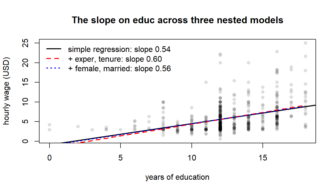
wage and educ under three nested specifications. The black line is the simple regression. The red dashed and blue dotted lines are the multiple-regression slopes (with controls fixed at sample means) for model2 and model3 respectively. Adding controls changes the slope on educ — this is the whole reason MLR exists. The shift from black to red is the magnitude of the OVB on educ from omitting experience and tenure.Compare goodness of fit across the three nested models:
Code
data.frame(
  model = c("educ only", "educ+exper+tenure", "full"),
  r2     = c(summary(model1)$r.squared,
             summary(model2)$r.squared,
             summary(model3)$r.squared),
  adj_r2 = c(summary(model1)$adj.r.squared,
             summary(model2)$adj.r.squared,
             summary(model3)$adj.r.squared)
)
model r2 adj_r2
1 educ only 0.1647575 0.1631635
2 educ+exper+tenure 0.3064224 0.3024364
3 full 0.3681887 0.3621136Both \(R^2\) and adjusted \(R^2\) rise as controls are added — here every added regressor is justified by labour-economics theory, so this should not surprise us.
3.11.2 Omitted variable bias on real data
Let us verify the OVB formula numerically. The “short” regression of wage on educ alone omits two regressors that we now know are correlated with education: exper and tenure. Run the two auxiliary regressions:
Code
aux_exper  <- lm(exper  ~ educ, data = wage1)
aux_tenure <- lm(tenure ~ educ, data = wage1)
delta_exper  <- coef(aux_exper)["educ"]
delta_tenure <- coef(aux_tenure)["educ"]
c(delta_exper = delta_exper, delta_tenure = delta_tenure)
delta_exper.educ delta_tenure.educ
-1.4681823 -0.1465559 The slope of exper on educ is negative: more-schooled workers in this 1976 cross-section have less labour-market experience (this is mostly mechanical — time spent in school is time not spent working). The slope of tenure on educ is slightly positive in this sample.
Now plug the auxiliary slopes and the long-regression coefficients into the OVB formula and compare with the actual gap between the short and long estimates:
Code
b1_short <- coef(model1)["educ"]
b1_long  <- coef(model2)["educ"]
b2_long  <- coef(model2)["exper"]
b3_long  <- coef(model2)["tenure"]

bias_predicted <- b2_long * delta_exper + b3_long * delta_tenure
bias_observed  <- b1_short - b1_long

c(predicted_bias = bias_predicted,
  observed_gap   = bias_observed)
predicted_bias.exper observed_gap.educ
-0.05760581 -0.05760581 The two numbers should coincide up to floating-point precision — this is the multivariable OVB extension stated in §3.9 (callout Extension: more than one omitted variable) at work, applied here to the two omitted regressors exper and tenure simultaneously. The simple-regression slope on educ differs from the multiple-regression slope by exactly \(\hat\beta_{\text{exper}}\tilde\delta_{\text{exper}} + \hat\beta_{\text{tenure}}\tilde\delta_{\text{tenure}}\).
What the numerical equality actually demonstrates is the Frisch–Waugh–Lovell sample identity — the sample slopes from short and long regressions are related by exactly the same algebraic combination as the population OVB formula, with \((\hat\beta, \tilde\delta)\) in place of \((\beta, \tilde\delta)\). The population OVB statement of §3.9 is the expected-value version of this sample identity; Exercise 3.6 asks you to derive the underlying FWL theorem.
NoteWhy the bias is negative here
Both exper and tenure have positive returns (\(\hat\beta_2, \hat\beta_3 > 0\)). But exper is negatively correlated with educ (\(\tilde\delta_{\text{exper}} < 0\)), and this dominates. The product \(\hat\beta_2\tilde\delta_{\text{exper}}\) is negative; omitting experience therefore drags the short-regression slope on educ downward relative to the long regression. The 2$$2 sign table above captures this exactly.
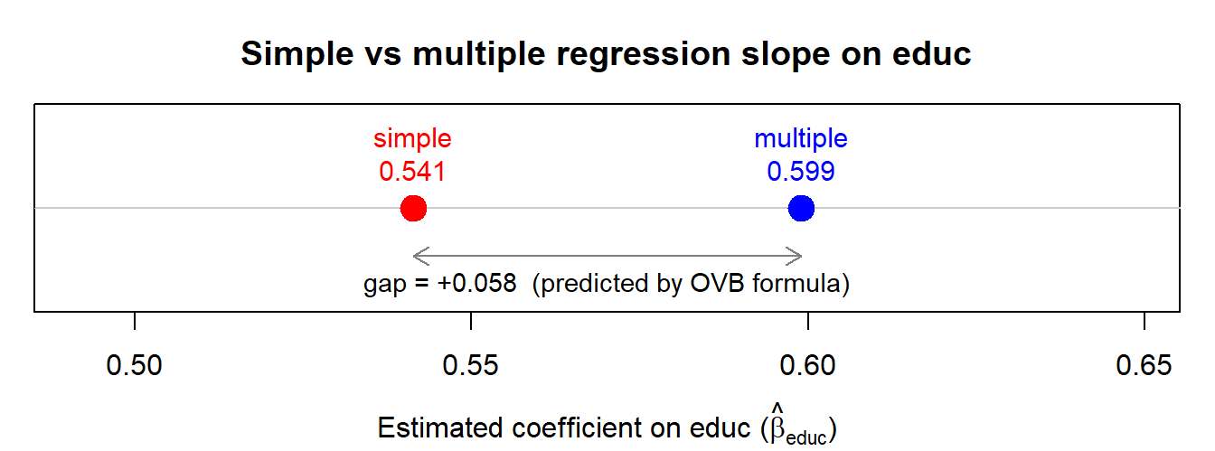
exper and tenure from a wage regression drags the educ coefficient downward in this sample. The gap between the two markers is exactly \(\hat\beta_{\text{exper}}\tilde\delta_{\text{exper}} + \hat\beta_{\text{tenure}}\tilde\delta_{\text{tenure}}\), the multivariable OVB formula at work.3.11.3 Perfect multicollinearity
Now a deliberate violation of MLR.3. Suppose we measure education in years (educ) and additionally create a redundant copy in months (educ_months = 12 * educ):
Code
wage1$educ_months <- 12 * wage1$educ
model_collinear <- lm(wage ~ educ + exper + tenure + educ_months, data = wage1)
summary(model_collinear)
Call:
lm(formula = wage ~ educ + exper + tenure + educ_months, data = wage1)

Residuals:
    Min      1Q  Median      3Q     Max
-7.6068 -1.7747 -0.6279  1.1969 14.6536

Coefficients: (1 not defined because of singularities)
            Estimate Std. Error t value Pr(>|t|)
(Intercept) -2.87273    0.72896  -3.941 9.22e-05 ***
educ         0.59897    0.05128  11.679  < 2e-16 ***
exper        0.02234    0.01206   1.853   0.0645 .
tenure       0.16927    0.02164   7.820 2.93e-14 ***
educ_months       NA         NA      NA       NA
---
Signif. codes:  0 '***' 0.001 '**' 0.01 '*' 0.05 '.' 0.1 ' ' 1

Residual standard error: 3.084 on 522 degrees of freedom
Multiple R-squared:  0.3064,    Adjusted R-squared:  0.3024
F-statistic: 76.87 on 3 and 522 DF,  p-value: < 2.2e-16
R does not crash — but it does silently drop educ_months (its coefficient is reported as NA). The reason is exactly MLR.3: educ_months is an exact linear function of educ, so the design matrix \(\mathbf{X}\) is rank-deficient, \(\mathbf{X}'\mathbf{X}\) is singular, and \((\mathbf{X}'\mathbf{X})^{-1}\) does not exist. We cannot tell whether a one-unit change in educ or a 12-unit change in educ_months is “doing the work” — the data simply does not contain that information.
WarningCommon mistake: the “168 minus hours” trap
A subtler version of the same problem: in a survey that records weekly hours worked (hours), one might be tempted to add a variable remaining = 168 - hours (“hours not worked in a week”, since 168 = 24$$7). The result is a perfect linear relationship between hours, remaining, and the constant: \(\text{hours} + \text{remaining} = 168\). Any regression including all three will be rank-deficient. The rule of thumb: if you can write one regressor as a deterministic function of the others (and the constant), you are in violation of MLR.3.
Self-check
Six short multiple-choice questions. Try each one before opening the answer.
TipQ1. Interpretation of an MLR slope
In the model \(y = \beta_0 + \beta_1 x_1 + \beta_2 x_2 + u\), the coefficient \(\beta_1\) measures:
- A. The total change in \(y\) when \(x_1\) goes up by one unit, including any indirect effect through \(x_2\).
- B. The expected change in \(y\) for a one-unit increase in \(x_1\), holding \(x_2\) fixed.
- C. The correlation between \(y\) and \(x_1\).
- D. The change in \(y\) when both \(x_1\) and \(x_2\) rise by one unit.
Answer: B. Every MLR slope is a partial effect: it isolates the variation in \(y\) associated with \(x_1\) once we hold the other regressors in the model constant.
TipQ2. The zero-conditional-mean assumption
MLR.4 requires:
- A. \(\operatorname{Cov}(x_1, u) = 0\) only.
- B. \(\operatorname{Var}(u\mid\mathbf{X}) = \sigma^2\).
- C. \(\mathbb{E}[u \mid x_1, x_2, \ldots, x_k] = 0\).
- D. \(u\) to be normally distributed.
Answer: C. MLR.4 is the conditional-mean-zero condition on all regressors simultaneously. It is what delivers unbiasedness of OLS.
TipQ3. Sign of OVB
In a wage regression we omit innate ability. Assume (i) more able workers earn more, holding education fixed, and (ii) more able workers acquire more education. The OLS coefficient on educ will be:
- A. Biased downward.
- B. Unbiased — OLS is always unbiased.
- C. Biased upward (overestimating the return to education).
- D. Of indeterminate sign.
Answer: C. With \(\beta_{\text{ability}} > 0\) and \(\tilde\delta_{\text{educ}} > 0\), the bias \(\beta_2\tilde\delta_1\) is positive: the short regression overstates the return to schooling.
TipQ4. Which assumption rules out perfect collinearity?
- A. MLR.1 (linearity in parameters).
- B. MLR.3 (no exact linear relationship among the regressors).
- C. MLR.4 (zero conditional mean).
- D. MLR.5 (homoskedasticity).
Answer: B. MLR.3 is the assumption that \(\mathbf{X}'\mathbf{X}\) is invertible. Violating it makes the OLS formula undefined; R will drop one of the offending variables and report NA.
TipQ5. \(R^2\) versus adjusted \(R^2\)
Which statement is true when an irrelevant regressor is added to a model?
- A. Both \(R^2\) and adjusted \(R^2\) always rise.
- B. \(R^2\) always rises (weakly), but adjusted \(R^2\) may fall.
- C. \(R^2\) may fall, but adjusted \(R^2\) always rises.
- D. Both always fall.
Answer: B. \(R^2\) cannot decrease because OLS could always set the new coefficient to zero. Adjusted \(R^2\) subtracts a penalty for parameters; if the new variable does not improve fit enough, the penalty wins.
TipQ6. When is OVB zero?
OVB on the slope of \(x_1\) is exactly zero when:
- A. The sample size is large.
- B. \(R^2\) exceeds 0.5.
- C. Either the omitted variable does not affect \(y\), or it is uncorrelated with \(x_1\).
- D. The errors are normal.
Answer: C. The OVB formula \(\beta_2\tilde\delta_1\) is zero whenever one of the two factors is zero. Large samples or high \(R^2\) do not fix omitted-variable bias.
Exercises
Exercise 3.1 ★ — Interpreting a fitted MLR. A researcher reports \[
\widehat{\text{wage}} = -2.87 + 0.599\,\text{educ} + 0.022\,\text{exper} + 0.169\,\text{tenure}
\] estimated on wage1. (a) Interpret each slope coefficient in plain English. (b) Predict the hourly wage of a worker with 16 years of education, 5 years of experience, and 3 years of tenure. (c) Why should you not read \(\hat\beta_1 = 0.599\) as the causal return to schooling?
TipShow answer
- Each slope is a partial effect: one additional year of education is associated with USD 0.60 more per hour, holding experience and tenure fixed; analogously for
experandtenure. (b) \(\widehat{\text{wage}} = -2.87 + 0.599\cdot 16 + 0.022\cdot 5 + 0.169\cdot 3 \approx 7.32\) USD/hour. (c) Because MLR.4 is unlikely to hold here — ability, family background, and school quality remain in \(u\) and are correlated witheduc. The slope is the best within-model linear summary, not a causal coefficient.
Exercise 3.2 ★ — Spotting perfect collinearity. For each of the following regressor sets, decide whether MLR.3 is violated. If so, identify the exact linear dependence.
{const, age, age_squared}.{const, female, male}, wheremale = 1 - female.{const, exper, tenure, exper + tenure}.{const, educ, log(educ)}— assumeeduc > 0.
TipShow answer
- No violation: \(\text{age}^2\) is not a linear function of
age. (b) Violation:female + male = 1, the constant column. (c) Violation: the fourth regressor is the sum of the second and third. (d) No violation: \(\log\) is nonlinear, so MLR.3 holds (though high collinearity may inflate variances).
Exercise 3.3 ★ — Sign of OVB from theory. You want to estimate the effect of class attendance on final grades but you omit student effort. Suppose effort raises grades and is positively correlated with attendance. Predict the sign of the bias on the coefficient of attendance in a short regression that omits effort, and explain in one sentence.
TipShow answer
With \(\beta_{\text{effort}} > 0\) and \(\tilde\delta_{\text{att}} > 0\), the bias \(\beta_2\tilde\delta_1\) is positive: the short regression overstates the return to attendance because part of the apparent effect is in fact the effect of the (unobserved) effort that correlates with attendance.
Exercise 3.4 ★ — Adjusted \(R^2\) falling. Construct a small numerical example (or argue analytically) showing that adding an irrelevant regressor can leave \(R^2\) essentially unchanged while making adjusted \(R^2\) smaller. Use the identity \(\bar R^2 = 1 - (n-1)(1-R^2)/(n-k-1)\) to explain why.
TipShow answer
With \(n = 100\), suppose \(R^2 = 0.30\) with \(k = 3\) regressors: \(\bar R^2 = 1 - 99\cdot 0.70/96 \approx 0.278\). Add an irrelevant 4th regressor that lifts \(R^2\) to \(0.301\): \(\bar R^2 = 1 - 99\cdot 0.699/95 \approx 0.272\). \(R^2\) went up by 0.001 but \(\bar R^2\) fell by 0.006 because \((n-1)/(n-k-1)\) grew faster than \(1-R^2\) shrank. This is the formal sense in which \(\bar R^2\) penalises complexity.
Exercise 3.5 ★★ — OVB by simulation. Generate \(n=1000\) observations from the model \(y = 1 + 2x_1 + 3x_2 + u\), where \(x_1 \sim \mathcal{N}(0,1)\), \(x_2 = 0.5\,x_1 + 0.5\,z\), \(z\sim\mathcal{N}(0,1)\) independent of \(x_1\), and \(u \sim \mathcal{N}(0,1)\) independent of everything else. (a) Estimate the short regression \(y\) on \(x_1\) alone and the long regression \(y\) on \((x_1, x_2)\). (b) Use the OVB formula to predict the gap between the two slopes on \(x_1\) and verify it numerically. Hint: \(\tilde\delta_1 = 0.5\) by construction.
A full answer is given in the Instructor Edition.
Exercise 3.6 ★★★ — Frisch–Waugh–Lovell partialling out. Let \(\tilde x_1\) denote the residuals from regressing \(x_1\) on the remaining regressors \((x_2,\ldots,x_k)\) and the constant. Show, using the OLS normal equations, that the multiple-regression coefficient on \(x_1\) equals the slope from a simple regression of \(y\) on \(\tilde x_1\). Verify your derivation numerically using wage1: regress educ on exper and tenure, keep the residuals, and check that regressing wage on those residuals reproduces \(\hat\beta_{\text{educ}}\) from the long regression of §3.10.
A full answer is given in the Instructor Edition.
Exercise 3.7 ★★ — The return to bwght. Chapter 2 §2.11 estimated a simple regression of birth weight on maternal smoking and warned that the slope on cigs might be contaminated by omitted variables (maternal income, education, nutrition). Use the multiple-regression toolkit to address that warning.
- Using
bwghtfrom the wooldridge package, estimate \[ \text{bwght} = \beta_0 + \beta_1\,\text{cigs} + \beta_2\,\text{motheduc} + \beta_3\,\text{fatheduc} + \beta_4\,\text{parity} + u. \] Report \(\hat\beta_1\) and compare it with the simple-regression slope \(-0.51\) from Ch 2 §2.11. Has it moved toward zero, away from zero, or stayed essentially the same? - Apply the multivariable OVB extension from §3.9. Run the three auxiliary regressions of
motheduc,fatheduc, andparityoncigs, and use the resulting \(\tilde\delta_j\) together with the long-regression coefficients \(\hat\beta_2, \hat\beta_3, \hat\beta_4\) to predict the gap between the simple- and multiple-regression slopes oncigs. Verify that your predicted gap matches the observed gap numerically (this is the FWL identity at work, exactly as in the wage example of §3.10.2). - Did including the controls change your causal interpretation of \(\hat\beta_1\) as the effect of maternal smoking on birth weight? Which assumption of MLR.1–MLR.4 are we still relying on, and which omitted variables remain to threaten it?
A full answer is given in the Instructor Edition.
Interactive self-assessment: LEARNR/03_multiple_linear_regression.Rmd.
Wooldridge, Jeffrey M. 2020. Introductory Econometrics: A Modern Approach. 7th ed. Cengage Learning.