4 Inference
Learning outcomes
By the end of this chapter the reader should be able to:
- State the Classical Linear Model assumptions (MLR.1–MLR.6) and explain what the normality assumption MLR.6 adds to Gauss–Markov.
- Derive the sampling distribution of \(\hat{\beta}_j\) under the CLM and explain why standardisation produces a \(t_{n-k-1}\) statistic rather than a standard normal.
- Construct and interpret a \((1-\alpha)\times 100\%\) confidence interval for an individual coefficient.
- Run a four-step hypothesis test (two-sided and one-sided) for a single coefficient, and read off the corresponding \(p\)-value.
- Carry out an \(F\)-test for joint significance, distinguishing the overall \(F\)-test from a restricted-vs-unrestricted comparison.
- Reproduce all of the above in R using
summary(),confint(),qt(),qf(),pt(),pf(),anova()and manual arithmetic on the fitted model.
Motivating empirical question
Once we hold education, experience and age fixed, do
IQscores and schooling jointly matter for monthly earnings — or could the apparent contribution of cognitive ability and education have arisen by chance?
We met IQ briefly in Chapter 3 as a candidate proxy for unobserved ability. Now we have to decide, formally, whether the coefficients we estimate are far enough from zero to take seriously. The tools of the chapter — \(t\)-statistics, \(p\)-values, confidence intervals and the \(F\)-test — are designed precisely for that decision.
4.1 From estimation to inference
2 and 3 produced point estimates \(\hat{\beta}_j\) from a sample. These numbers are random: a different sample would have given different numbers. The question of inference is whether what we learned from our sample lets us say anything credible about the unknown population parameter \(\beta_j\).
Statistical inference provides two complementary tools (Wooldridge 2020):
- Confidence intervals. A range of plausible values for the unknown parameter, with a calibrated long-run coverage probability.
- Hypothesis tests. A formal procedure for deciding whether the data are compatible with a specific claim about the parameter — most often, the claim that the parameter equals zero.
Both tools rely on knowing the sampling distribution of \(\hat{\beta}_j\). Under Gauss–Markov we only know its mean (\(\beta_j\)) and variance; we do not know its shape. To say anything precise about probabilities — “the chance of observing a coefficient this far from zero, if the truth is zero, is less than 1%” — we need a distribution. That is what the next assumption gives us.
4.2 The Classical Linear Model (CLM) assumptions
Gauss–Markov gave us unbiasedness, a closed-form variance and the BLUE property of OLS. For exact (finite-sample) inference we need one more assumption.
NoteDefinition: MLR.6 (Normality of the error term)
Conditional on the regressors \(\mathbf{X}\), the population error \(u\) is normally distributed with mean zero and constant variance:
\[ u \mid \mathbf{X} \;\sim\; \mathcal{N}(0,\,\sigma^2). \]
The full set MLR.1–MLR.6 is called the Classical Linear Model (CLM) assumptions.
Why normality, and where does it come from? In many applied settings \(u\) is the additive sum of a large number of small, independent omitted factors, and a central-limit heuristic suggests its distribution should be roughly bell-shaped. The qualifier “additive” matters: the heuristic does not survive if the omitted factors combine multiplicatively. The assumption is strong: it can fail badly for skewed outcomes such as wages or counts. We will see in Chapter 6 that taking \(\log\) of the dependent variable is precisely the trick that converts multiplicative omitted factors into additive ones, which is one reason logs so often make the residuals look symmetric.
The pay-off is large. Under MLR.1–MLR.6, the OLS estimator inherits the normality of \(u\):
\[ \hat{\beta}_j \mid \mathbf{X} \;\sim\; \mathcal{N}\!\left(\beta_j,\,\operatorname{Var}(\hat{\beta}_j)\right). \]
This is an exact statement that holds in any sample size, not just asymptotically. With \(n\) large, the central limit theorem delivers approximately the same conclusion even without MLR.6, but only the CLM gives us exact small-sample inference.
WarningCommon mistake: confusing the normality of \(u\) with the normality of \(y\)
MLR.6 is a statement about the error \(u\), conditional on the regressors. It is not the claim that the marginal distribution of \(y\) is normal. Wages, for example, are right-skewed; that does not by itself contradict MLR.6, because the systematic component \(\beta_0 + \beta_1 x_1 + \cdots\) can absorb the skewness.
4.3 The \(t\)-distribution
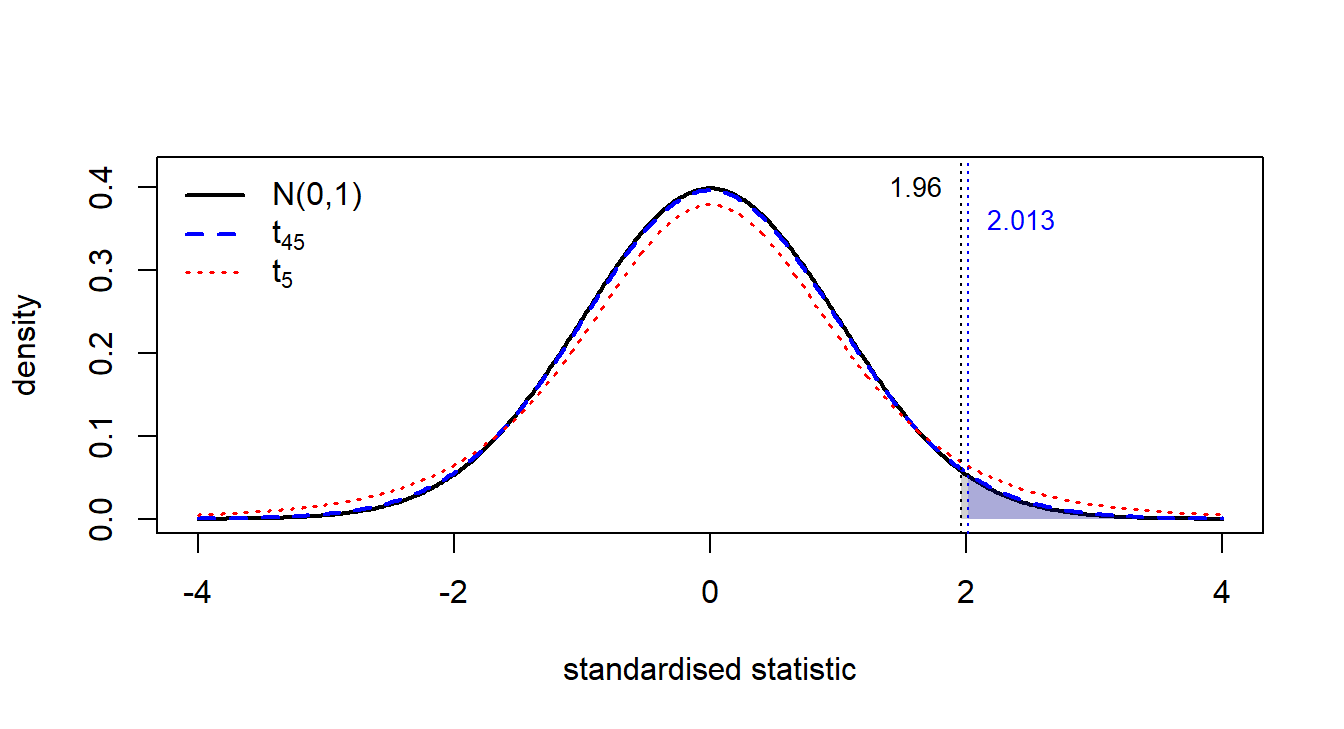
Imagine for a moment that we knew the true error variance \(\sigma^2\). Then dividing \(\hat{\beta}_j - \beta_j\) by its (known) standard deviation would give a clean standard-normal \(Z\): one random quantity divided by a fixed constant. In reality we do not know \(\sigma^2\); we replace it with the sample estimate \(\hat{\sigma}^2 = \mathrm{SSR}/(n-k-1)\). The crucial observation is that \(\hat{\sigma}\) is itself a random number — different samples produce different \(\hat{\sigma}\) values. So the standardised ratio is no longer a random quantity over a constant, but a random quantity over another random quantity, which is necessarily more variable than \(Z\). The extra variability shows up as heavier tails: the resulting distribution is the \(t\)-distribution, narrower at the centre and fatter in the tails than the standard normal (see the figure below comparing \(t_{45}\), \(t_5\), and \(\mathcal{N}(0,1)\)).
Made formal: if \(\sigma^2\) were known we would have
\[ Z \;=\; \frac{\hat{\beta}_j - \beta_j}{\sqrt{\operatorname{Var}(\hat{\beta}_j)}} \;\sim\; \mathcal{N}(0,1). \]
In practice \(\sigma^2\) is unknown, \(\hat{\sigma}^2\) takes its place in the standard error, and the standardised statistic is no longer standard normal: it is \(t\)-distributed with \(n-k-1\) degrees of freedom,
\[ t \;=\; \frac{\hat{\beta}_j - \beta_j}{\operatorname{se}(\hat{\beta}_j)} \;\sim\; t_{\,n-k-1}. \]
The \(t\)-distribution is symmetric, bell-shaped and centred at zero, but it has heavier tails than \(\mathcal{N}(0,1)\) — a reflection of the extra uncertainty from estimating \(\sigma^2\). As the degrees of freedom \(n-k-1\) grow, the tails thin out and \(t_{n-k-1}\) converges to \(\mathcal{N}(0,1)\). For \(n-k-1 \geq 120\) the two distributions are virtually indistinguishable; for small samples the \(t\) is noticeably wider.
That is the whole reason this chapter uses \(t\) critical values like \(2.013\) (for \(\alpha = 0.05\), \(df = 45\)) rather than the familiar \(1.96\) from the normal table.
4.4 Two ways to be wrong
A jury can convict an innocent defendant, or it can let a guilty one go free. Both mistakes are bad and the legal system is built to trade them off. A hypothesis test faces exactly the same two-by-two structure.
| \(H_0\) is true | \(H_0\) is false | |
|---|---|---|
| Reject \(H_0\) | Type I error (size \(\alpha\)) | Correct rejection (power \(1-\beta\)) |
| Fail to reject \(H_0\) | Correct non-rejection | Type II error (probability \(\beta\)) |
A Type I error is rejecting a null that is in fact true — the statistical equivalent of convicting an innocent defendant. The probability of making one, computed under \(H_0\), is called the size of the test:
\[ \alpha \;=\; \Pr\bigl(\text{reject } H_0 \,\big|\, H_0 \text{ true}\bigr). \]
The conventional choices \(\alpha = 0.10, 0.05, 0.01\) are precisely the Type I error rates we are willing to tolerate. Notice the conditional: \(\alpha\) is not the probability that the null is true given the data, nor the probability that we will reject in any given study. It is the long-run frequency of false rejections across studies where the null happens to be true.
A Type II error is failing to reject a null that is in fact false — the equivalent of letting a guilty defendant go free. Its probability is denoted \(\beta\). The complement, \(1 - \beta\), is the power of the test: the probability of detecting a real effect when one exists. Unlike \(\alpha\), power depends on three things: how large the true effect is, how noisy the data are, and how many observations we have. Underpowered studies miss real effects routinely; this is why a “non-significant” finding in a small sample is rarely informative.
There is no free lunch. Holding \(n\) and the data-generating process fixed, lowering \(\alpha\) (a stricter test) raises \(\beta\) (more missed real effects), and vice versa. The only way to reduce both error probabilities simultaneously is to gather more data — which makes the sampling distribution under \(H_0\) tighter and shrinks both tails.
WarningCommon mistake: confusing \(\alpha\) with \(p\), and “size” with “significance”
The size \(\alpha\) is set before the data are seen — it is the long-run Type I error rate we are willing to accept. The \(p\)-value is computed after the data are seen — it is the smallest \(\alpha\) at which the data would lead us to reject. The two are distinct conceptual objects even though they share the same scale. Similarly, the “5% significance level” in a paper refers to a chosen \(\alpha\), not to a per-study probability of error: each individual study either rejected correctly or did not, and we will never know which.
We will use the vocabulary of “size” and “power” repeatedly below — particularly in §“\(F\)-test for joint significance,” where the size of a combined procedure (testing several restrictions at once) is precisely what motivates the \(F\)-test in the first place.
4.5 Confidence intervals
NoteDefinition: confidence interval for \(\beta_j\)
A \((1-\alpha)\times 100\%\) confidence interval for \(\beta_j\) is
\[ \hat{\beta}_j \;\pm\; t_{\alpha/2,\,n-k-1}\,\cdot\,\operatorname{se}(\hat{\beta}_j), \]
where \(t_{\alpha/2,\,n-k-1}\) is the critical value of the \(t\)-distribution that leaves probability \(\alpha/2\) in each tail.
For the canonical 95% interval, \(\alpha = 0.05\) and the critical value is \(t_{0.025,\,n-k-1}\). With moderately large samples this is close to \(1.96\), but in small samples it can be appreciably larger.
WarningCommon mistake: misreading the “95%”
A 95% confidence interval is a statement about the procedure, not about the realised interval. If we drew many independent samples and built one interval from each, about 95% of those intervals would contain the true \(\beta_j\). It is not correct to say that there is a 95% probability that the particular interval \([L, U]\) we computed from our one sample contains \(\beta_j\) — \(\beta_j\) is a fixed (if unknown) number, and the realised interval either covers it or it does not.
Confidence intervals and two-sided hypothesis tests are two sides of the same coin: a \((1-\alpha)\) CI for \(\beta_j\) contains zero if and only if the two-sided \(t\)-test of \(H_0:\beta_j = 0\) at level \(\alpha\) fails to reject.
4.6 Hypothesis testing in four steps
We test claims about a single coefficient \(\beta_j\) using a standard four-step procedure. Let \(c\) be the hypothesised value (usually \(c = 0\), “the variable does not matter”).
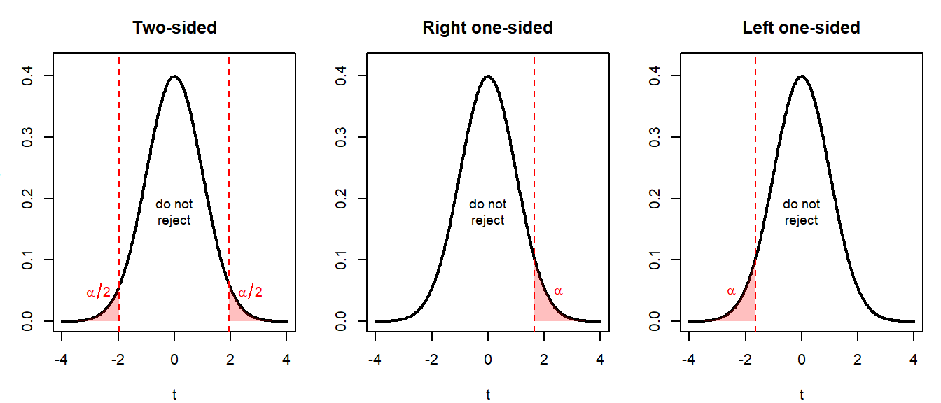
Step 1. State \(H_0\) and \(H_1\). There are three useful forms:
- Two-sided: \(H_0: \beta_j = c\) versus \(H_1: \beta_j \neq c\).
- Right one-sided: \(H_0: \beta_j \leq c\) versus \(H_1: \beta_j > c\).
- Left one-sided: \(H_0: \beta_j \geq c\) versus \(H_1: \beta_j < c\).
The choice between one- and two-sided is driven by economic theory, not by the data: if theory tells us a priori that \(\beta_j\) cannot be negative, a one-sided test is appropriate.
Step 2. Choose a significance level \(\alpha\) and read off the critical value. Standard choices are \(\alpha = 0.10\), \(0.05\), \(0.01\). The critical value is
- \(t_{\alpha/2,\,n-k-1}\) for a two-sided test,
- \(t_{\alpha,\,n-k-1}\) for a one-sided test.
Step 3. Compute the \(t\)-statistic.
\[ t \;=\; \frac{\hat{\beta}_j - c}{\operatorname{se}(\hat{\beta}_j)}. \]
For the default \(c = 0\) this reduces to \(t = \hat{\beta}_j / \operatorname{se}(\hat{\beta}_j)\), which is exactly the number R reports in the third column of summary(lm(...)).
Step 4. Compare and conclude.
- Two-sided: reject \(H_0\) if \(|t| > t_{\alpha/2,\,n-k-1}\).
- Right one-sided: reject \(H_0\) if \(t > t_{\alpha,\,n-k-1}\).
- Left one-sided: reject \(H_0\) if \(t < -t_{\alpha,\,n-k-1}\).
If \(H_0\) is rejected we say the coefficient is statistically significant at the chosen level. If we fail to reject we say the data are consistent with \(H_0\) — we never “accept” \(H_0\), because the test was designed to detect departures from it, not to confirm it.
WarningCommon mistake: statistical significance is not economic significance
A coefficient can be statistically significant (small \(p\)-value) but economically tiny, and a coefficient can be economically large but statistically insignificant in a small sample. Always report both: the magnitude of \(\hat{\beta}_j\) in the units of the problem, and the precision with which it is estimated. A 1% return to one extra year of education and a 10% return are both “significantly different from zero” in a large sample, but only one of them is policy-relevant.
4.7 The \(p\)-value
The four-step procedure forces us to fix \(\alpha\) in advance. A more informative alternative is to report the \(p\)-value.
NoteDefinition: \(p\)-value
The \(p\)-value is the probability, computed under \(H_0\), of observing a test statistic at least as extreme as the one we got. Equivalently, it is the smallest significance level \(\alpha\) at which we would reject \(H_0\).
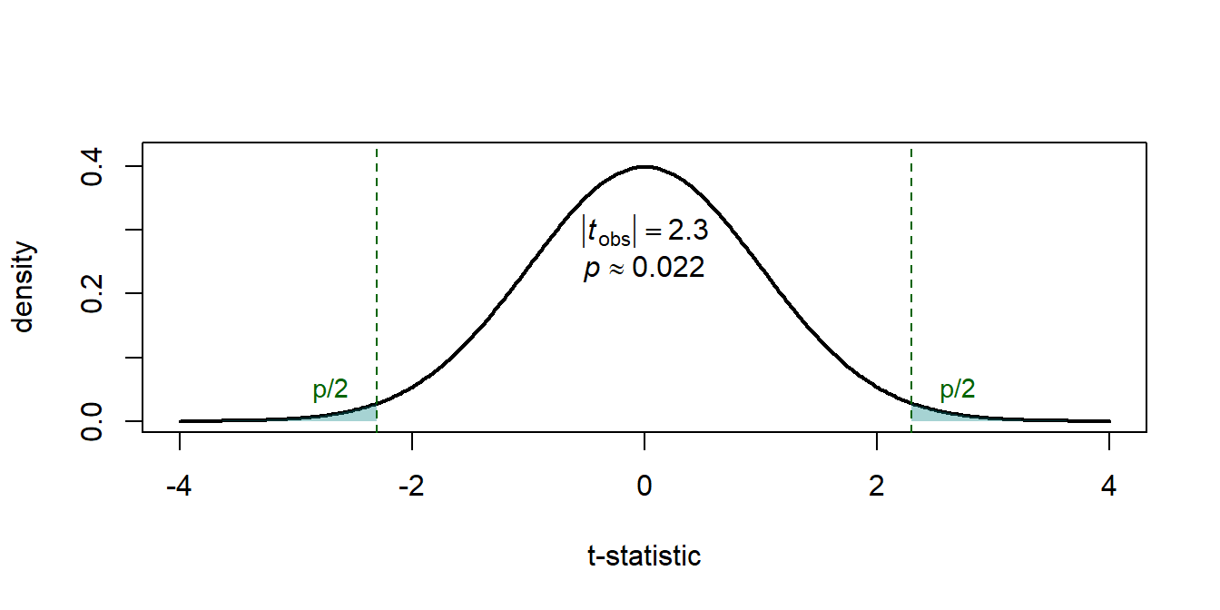
For a two-sided test of \(H_0:\beta_j = 0\) with computed statistic \(t\),
\[ p \;=\; 2 \cdot \Pr\!\left(T_{n-k-1} > |t|\right) \;=\; 2\,\bigl[1 - F_t(|t|;\,n-k-1)\bigr], \]
where \(F_t\) is the CDF of the \(t_{n-k-1}\) distribution. For a one-sided test the \(p\)-value is exactly half of this (when the sign of \(\hat{\beta}_j\) agrees with the alternative).
Conventional rules of thumb (Wooldridge 2020):
- \(p < 0.01\): strong evidence against \(H_0\) (reject at the 1% level).
- \(p < 0.05\): evidence against \(H_0\) (reject at the 5% level).
- \(p < 0.10\): weak evidence against \(H_0\) (reject at the 10% level).
- \(p \geq 0.10\): insufficient evidence to reject \(H_0\).
R reports two-sided \(p\)-values by default in the Pr(>|t|) column of summary(lm(...)), together with significance stars: *** for \(p < 0.001\), ** for \(p < 0.01\), * for \(p < 0.05\), . for \(p < 0.10\).
WarningCommon mistake: a small \(p\)-value is not a causal certificate
Statistical significance tells us that \(\hat{\beta}_j\) is unlikely to have arisen by sampling noise if the truth were zero. It says nothing about whether \(x_j\) causes \(y\). Causal interpretation still requires the population assumption \(\mathbb{E}[u \mid \mathbf{X}] = 0\) (MLR.4) — no \(p\)-value, however small, can rescue a regression contaminated by omitted-variable bias or by reverse causality.
4.8 The \(F\)-test for joint significance
Recall the opening question of this chapter: do IQ and educ jointly matter for monthly earnings? This is precisely the kind of joint hypothesis the \(F\)-test was built for.
Single-coefficient \(t\)-tests are the right tool when we have one parameter in mind. Often, though, the question is whether several coefficients are jointly zero:
- “Are
educandIQjointly irrelevant for wages once we control for hours, experience and age?” - “Do the squared terms in a polynomial in
experadd anything to the model?” - “Do any of the regressors matter — is the overall regression worth running?”
These are joint hypotheses, and they require a joint test. Doing \(q\) separate \(t\)-tests does not answer the joint question, for two reasons. First, each individual \(t\)-test has size \(\alpha\), but the combined procedure — “reject the joint null if any individual \(t\)-test rejects” — has a Type I error rate that grows with the number of comparisons. With \(q = 2\) independent tests each at size \(0.05\), the overall probability of rejecting at least one true null is roughly \(1 - (1 - 0.05)^2 \approx 0.10\), not \(0.05\). Second, two coefficients can be jointly informative even when each is individually borderline; running them separately throws away the information in their combination.
4.8.1 Restricted vs unrestricted models
Let the unrestricted model be the regression with \(k\) slopes,
\[ y = \beta_0 + \beta_1 x_1 + \cdots + \beta_k x_k + u. \]
Suppose we want to test that the last \(q\) slopes are zero,
\[ H_0:\;\beta_{k-q+1} = \beta_{k-q+2} = \cdots = \beta_k = 0, \]
against the alternative that at least one of them is non-zero. The restricted model imposes \(H_0\) by dropping those \(q\) regressors:
\[ y = \beta_0 + \beta_1 x_1 + \cdots + \beta_{k-q} x_{k-q} + u. \]
Let \(\mathrm{SSR}_U\) and \(\mathrm{SSR}_R\) denote the sum of squared residuals of the unrestricted and restricted models. Because dropping regressors can never reduce the SSR, we always have \(\mathrm{SSR}_R \geq \mathrm{SSR}_U\); the question is whether the gap is big enough to be inconsistent with \(H_0\).
NoteDefinition: the \(F\)-statistic
Under \(H_0\) and MLR.1–MLR.6,
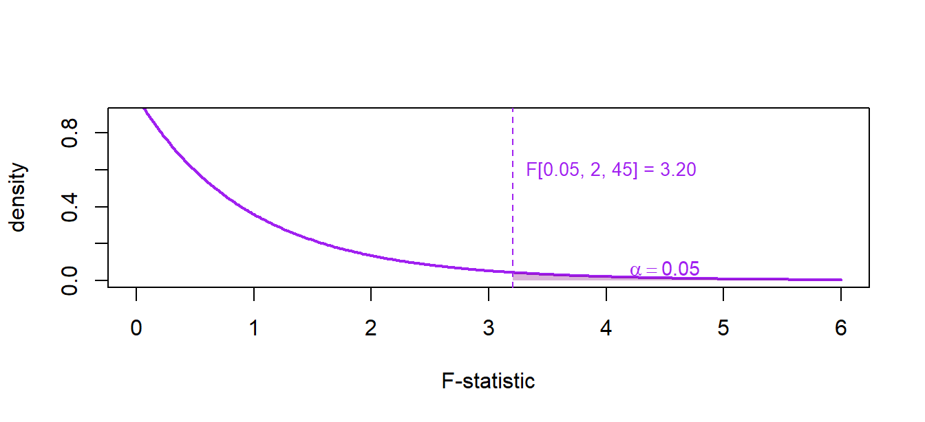
\[ F \;=\; \frac{(\mathrm{SSR}_R - \mathrm{SSR}_U)/q}{\mathrm{SSR}_U/(n-k-1)} \;\sim\; F_{q,\,n-k-1}. \]
Reject \(H_0\) at level \(\alpha\) if \(F > F_{q,\,n-k-1,\,\alpha}\), the upper-\(\alpha\) critical value of the \(F\) distribution with \(q\) and \(n-k-1\) degrees of freedom.
An equivalent formulation uses the \(R^2\) of each model:
\[ F \;=\; \frac{(R^2_U - R^2_R)/q}{(1 - R^2_U)/(n-k-1)}. \]
The two formulas are algebraically identical whenever \(y\) is the same in both regressions.
WarningCommon mistake: \(F\) across different dependent variables
Both the SSR-based and the \(R^2\)-based formulas require the same dependent variable in the restricted and unrestricted models. If \(y\) differs between models — the classic case is testing \(\log y\) against \(y\) — neither \(\mathrm{SSR}_R - \mathrm{SSR}_U\) nor \(R^2_U - R^2_R\) is on a comparable scale, and the \(F\)-statistic computed by either formula is meaningless — not just imprecise. Tests across non-nested specifications with different left-hand-side variables require different machinery (e.g. the Vuong test or Davidson–MacKinnon \(J\)-test), which is beyond the scope of this chapter.
4.8.2 The overall \(F\)-test
A special case is the test that every slope is zero,
\[ H_0:\;\beta_1 = \beta_2 = \cdots = \beta_k = 0. \]
Here the restricted model is the regression on a constant alone, and \(R^2_R = 0\). The \(F\)-statistic collapses to
\[ F \;=\; \frac{R^2/k}{(1-R^2)/(n-k-1)}, \]
which is exactly the number R prints at the bottom line of summary(lm(...)) under “F-statistic”, together with its \(p\)-value.
4.8.3 \(F\) versus \(t\): a useful identity
For a single restriction (\(q = 1\)), the \(F\)-statistic equals the square of the corresponding \(t\)-statistic:
\[ F \;=\; t^2, \qquad F_{1,\,n-k-1} \;=\; \bigl(t_{n-k-1}\bigr)^2. \]
The \(t\)- and \(F\)-tests deliver identical conclusions in this case; the \(F\) machinery is only strictly necessary when \(q \geq 2\).
4.9 Lab: inference
NoteNotation reminder
Throughout this chapter, \(k\) denotes the number of slope coefficients (matching the Wooldridge convention), so the unrestricted model has \(k+1\) parameters and \(n - k - 1\) residual degrees of freedom. Some textbooks reserve \(k\) for the total number of parameters including the intercept; mixing the two conventions silently shifts every degrees-of-freedom count by one and gives wrong critical values. Keep Wooldridge’s convention throughout this lab.
We work with wage2 from the wooldridge package: a cross-section of \(n = 935\) U.S. men in the 1980 National Longitudinal Survey, with information on monthly earnings (wage), weekly hours (hours), an IQ test score (IQ), years of schooling (educ), years of work experience (exper), tenure with the current employer (tenure) and age. The goal is to translate the four-step inference machinery into R commands and then check that the built-in shortcuts give the same answers.
Code
library(wooldridge)
data("wage2")
4.9.1 A first regression and its summary()
Start with a simple regression of monthly wage on weekly hours:
Code
model1 <- lm(wage ~ hours, data = wage2)
summary(model1)
Call:
lm(formula = wage ~ hours, data = wage2)

Residuals:
    Min      1Q  Median      3Q     Max
-839.72 -287.21  -52.38  200.46 2131.26

Coefficients:
            Estimate Std. Error t value Pr(>|t|)
(Intercept)  981.315     81.575   12.03   <2e-16 ***
hours         -0.532      1.832   -0.29    0.772
---
Signif. codes:  0 '***' 0.001 '**' 0.01 '*' 0.05 '.' 0.1 ' ' 1

Residual standard error: 404.6 on 933 degrees of freedom
Multiple R-squared:  9.033e-05, Adjusted R-squared:  -0.0009814
F-statistic: 0.08429 on 1 and 933 DF,  p-value: 0.7716
The summary() block reports, for each coefficient, the estimate \(\hat{\beta}_j\), its standard error \(\operatorname{se}(\hat{\beta}_j)\), the \(t\)-statistic \(\hat{\beta}_j/\operatorname{se}(\hat{\beta}_j)\), and the two-sided \(p\)-value. At the bottom we see the overall \(F\)-statistic and its \(p\)-value, which test \(H_0: \beta_{\text{hours}} = 0\) in this single-regressor case.
Now move to a richer specification:
Code
model2 <- lm(wage ~ hours + educ + exper + IQ + age, data = wage2)
summary(model2)
Call:
lm(formula = wage ~ hours + educ + exper + IQ + age, data = wage2)

Residuals:
    Min      1Q  Median      3Q     Max
-883.49 -238.11  -47.36  190.09 2144.24

Coefficients:
             Estimate Std. Error t value Pr(>|t|)
(Intercept) -778.4403   171.2506  -4.546 6.20e-06 ***
hours         -2.5406     1.6811  -1.511  0.13104
educ          52.4505     7.2981   7.187 1.36e-12 ***
exper         10.9390     3.7196   2.941  0.00335 **
IQ             5.2917     0.9383   5.640 2.26e-08 ***
age           14.4836     4.6657   3.104  0.00197 **
---
Signif. codes:  0 '***' 0.001 '**' 0.01 '*' 0.05 '.' 0.1 ' ' 1

Residual standard error: 368.9 on 929 degrees of freedom
Multiple R-squared:  0.1722,    Adjusted R-squared:  0.1678
F-statistic: 38.66 on 5 and 929 DF,  p-value: < 2.2e-16
NoteReading the
summary() output — columns that now carry the load
In Chapters 2 and 3 we labelled each summary() column but pointed the student to “we’ll come back to t and p in Ch 4.” This is that chapter. The columns that were ornamental in Ch 2 are doing the inferential work now.
Estimate→ \(\hat\beta_j\), the OLS coefficient.Std. Error→ \(\operatorname{se}(\hat\beta_j)\), the square root of the appropriate diagonal of \(\hat\sigma^2 (\mathbf{X}'\mathbf{X})^{-1}\).t value→ \(t = \hat\beta_j / \operatorname{se}(\hat\beta_j)\), the test statistic for \(H_0: \beta_j = 0\) that we built in §4.3. Under MLR.1–MLR.6, it follows \(t_{n-k-1}\).Pr(>|t|)→ the two-sided \(p\)-value defined in §4.7. With \(\alpha = 0.05\) as the conventional cutoff, anything in this column below 0.05 corresponds to a “statistically significant” coefficient.- The
Signif. codesline interpretsPr(>|t|)with stars:***\(p < 0.001\),**\(p < 0.01\),*\(p < 0.05\),.\(p < 0.10\). Residual standard error: X on Y degrees of freedom→ \(\hat\sigma\), with \(Y = n - k - 1\) residual degrees of freedom (here \(n - 5 - 1\)).Multiple R-squared/Adjusted R-squared→ \(R^2\) and \(\bar R^2\) from §3.8.- Bottom line
F-statistic: X on Df1 and Df2 DF, p-value: Y→ this is the overall \(F\)-test of §4.8.2, which tests \(H_0: \beta_1 = \beta_2 = \cdots = \beta_k = 0\) (every slope is zero).Df1 = k,Df2 = n - k - 1, and thep-valueis the right-tail probability under \(F_{k, n-k-1}\).
Read the table line by line: educ and IQ both have large \(t\)-statistics and tiny \(p\)-values, so each is individually significant at the 1% level even after controlling for the others. hours is negative and significant (men who work longer hours earn slightly less per week of hours worked, conditional on the other covariates — a hint that hours are correlated with occupational mix). exper and age are statistically indistinguishable from zero in this specification.
4.9.2 Manual confidence intervals with qt()
Pull out the coefficients and standard errors programmatically, then build a 95% CI by hand.
Code
beta_hat <- coef(model2)
se_hat   <- summary(model2)$coefficients[, "Std. Error"]

n  <- nobs(model2)
k  <- length(beta_hat) - 1     # number of slope coefficients
df <- n - k - 1

t_crit <- qt(0.975, df)
t_crit                           # critical value t_{0.025, df}
[1] 1.962521The critical value is close to \(1.96\) because the degrees of freedom are large, but not identical. The manual 95% CI for \(\beta_{\text{IQ}}\) is
Code
IQ_LB <- beta_hat["IQ"] - t_crit * se_hat["IQ"]
IQ_UB <- beta_hat["IQ"] + t_crit * se_hat["IQ"]
c(lower = IQ_LB, upper = IQ_UB)
lower.IQ upper.IQ
3.450211 7.133145 and for \(\beta_{\text{hours}}\):
Code
hours_LB <- beta_hat["hours"] - t_crit * se_hat["hours"]
hours_UB <- beta_hat["hours"] + t_crit * se_hat["hours"]
c(lower = hours_LB, upper = hours_UB)
lower.hours upper.hours
-5.8397528 0.7584696 The built-in shortcut delivers all the intervals in one call:
Code
confint(model2, level = 0.95) 2.5 % 97.5 %
(Intercept) -1114.523218 -442.3574662
hours -5.839753 0.7584696
educ 38.127749 66.7731627
exper 3.639234 18.2387119
IQ 3.450211 7.1331452
age 5.327113 23.6400802The numbers in the IQ and hours rows match what we computed by hand. Notice that the 95% interval for IQ excludes zero (consistent with the small \(p\)-value in the summary()), while the intervals for exper and age do contain zero (consistent with their non-significance).
4.9.3 Manual \(t\)-test for a single coefficient
Suppose we want to test \(H_0: \beta_{\text{educ}} = 0\) against the two-sided alternative at the 5% level. Step by step:
Code
b_educ  <- coef(model2)["educ"]
se_educ <- summary(model2)$coefficients["educ", "Std. Error"]

t_stat  <- b_educ / se_educ
p_value <- 2 * pt(-abs(t_stat), df)   # two-sided p-value

c(t = t_stat, p = p_value)
t.educ p.educ
7.186848e+00 1.361083e-12 Code
summary(model2)$coefficients["educ", c("t value", "Pr(>|t|)")] t value Pr(>|t|)
7.186848e+00 1.361083e-12 The bottom two lines are identical (up to rounding): the manual computation reproduces exactly what R prints. The \(t\)-statistic is far above the 5% critical value of roughly \(1.96\), so we reject \(H_0\). Education has a statistically significant partial effect on monthly earnings even after controlling for hours, experience, IQ and age.
4.9.4 Manual \(F\)-test for joint significance
Now the headline question of the chapter: are educ and IQ jointly relevant once hours, exper and age are in the model? Formally,
\[ H_0:\;\beta_{\text{educ}} = \beta_{\text{IQ}} = 0 \quad\text{vs.}\quad H_1:\;\text{at least one of them }\neq 0, \]
so \(q = 2\).
The unrestricted model is model2 above. The restricted model drops educ and IQ:
Code
model3 <- lm(wage ~ hours + exper + age, data = wage2)
summary(model3)
Call:
lm(formula = wage ~ hours + exper + age, data = wage2)

Residuals:
    Min      1Q  Median      3Q     Max
-749.69 -279.16  -48.16  203.20 2208.66

Coefficients:
            Estimate Std. Error t value Pr(>|t|)
(Intercept)  224.411    162.071   1.385  0.16649
hours         -1.175      1.812  -0.649  0.51665
exper         -9.430      3.443  -2.739  0.00628 **
age           27.032      4.838   5.587 3.03e-08 ***
---
Signif. codes:  0 '***' 0.001 '**' 0.01 '*' 0.05 '.' 0.1 ' ' 1

Residual standard error: 398.4 on 931 degrees of freedom
Multiple R-squared:  0.03253,   Adjusted R-squared:  0.02941
F-statistic: 10.44 on 3 and 931 DF,  p-value: 9.332e-07
Compute the SSRs by hand:
Code
SSR_u <- sum(residuals(model2)^2)
SSR_r <- sum(residuals(model3)^2)
c(SSR_unrestricted = SSR_u, SSR_restricted = SSR_r)
SSR_unrestricted SSR_restricted
126414757 147747973 Now the \(F\)-statistic:
Code
q    <- 2                # restrictions
df_u <- n - k - 1        # df of the unrestricted model

F_stat <- ((SSR_r - SSR_u) / q) / (SSR_u / df_u)
F_crit <- qf(0.95, df1 = q, df2 = df_u)
p_val  <- 1 - pf(F_stat, df1 = q, df2 = df_u)

c(F = F_stat, F_crit_5pct = F_crit, p = p_val)
F F_crit_5pct p
78.387043 3.005413 0.000000 The \(F\)-statistic is far above the 5% critical value and the \(p\)-value is essentially zero, so we strongly reject \(H_0\): educ and IQ are jointly significant determinants of wage.
R provides the same test in one line via anova(), which compares two nested models:
Code
anova(model3, model2)Analysis of Variance Table
Model 1: wage ~ hours + exper + age
Model 2: wage ~ hours + educ + exper + IQ + age
Res.Df RSS Df Sum of Sq F Pr(>F)
1 931 147747973
2 929 126414757 2 21333216 78.387 < 2.2e-16 ***
---
Signif. codes: 0 '***' 0.001 '**' 0.01 '*' 0.05 '.' 0.1 ' ' 1
NoteReading the
anova() output — model comparison columns
anova(restricted, unrestricted) prints a two-row table. Row 1 is the restricted model, row 2 the unrestricted. The columns map directly to the \(F\)-formula:
Res.Dfrow 2 → \(n - k - 1\) = residual degrees of freedom of the unrestricted model (the denominator df of the \(F\) in §4.8).Res.Dfrow 1 → \(n - (k - q) - 1\) for the restricted model; equivalently,Res.Dfrow 1 \(-\)Res.Dfrow 2 \(= q\) (the number of restrictions).RSS→ \(\mathrm{SSR}\) for each model (R calls it “residual sum of squares”).Dfrow 2 → \(q\), the number of restrictions being tested.Sum of Sqrow 2 → \(\mathrm{SSR}_R - \mathrm{SSR}_U\), the gain in residual SSR that comes from dropping \(q\) regressors.Frow 2 → the \(F\)-statistic itself: \(\bigl[(\mathrm{SSR}_R - \mathrm{SSR}_U)/q\bigr] / \bigl[\mathrm{SSR}_U/(n - k - 1)\bigr]\).Pr(>F)row 2 → the right-tail \(p\)-value under \(F_{q, n-k-1}\).
The F and Pr(>F) columns reproduce the manual computation. Reporting the \(F\)-test from anova() is the recommended workflow; the manual derivation matters because it lets you see exactly what is being compared.
4.9.5 \(F = t^2\) in a single-restriction test
The identity at the end of §4.7 is easy to verify numerically. Test \(H_0: \beta_{\text{educ}} = 0\) both ways:
Code
t_educ <- summary(model2)$coefficients["educ", "t value"]

mR <- lm(wage ~ hours + exper + IQ + age, data = wage2)   # drop educ only
ft <- anova(mR, model2)
F_single <- ft$F[2]

c(t_squared = t_educ^2, F = F_single)
t_squared F
51.65078 51.65078 The two numbers agree, as the algebra predicts.
4.9.6 One-sided vs two-sided
Suppose theory tells us that an extra year of experience cannot lower monthly earnings, so the relevant alternative is right-sided: \(H_0: \beta_{\text{exper}} \leq 0\) vs \(H_1: \beta_{\text{exper}} > 0\). The same \(t\)-statistic feeds a different \(p\)-value:
Code
co <- summary(model2)$coefficients["exper", ]
t_exper <- co["t value"]

p_one_sided <- if (t_exper > 0) 1 - pt(t_exper, df) else 1
# ^ right-tail p-value. Only meaningful when the estimate is already on the
#   side of the alternative (t_exper > 0 here). If the estimate had the
#   wrong sign for a right-sided alternative, the correct one-sided p-value
#   would be ~1 ("no evidence in the alternative's direction"), NOT the
#   naive 1 - pt(t_exper, df), which would return a value above 0.5.
p_two_sided <- 2 * pt(-abs(t_exper), df)   # default in summary()

c(t = t_exper, p_one_sided = p_one_sided, p_two_sided = p_two_sided)
t.t value p_one_sided.t value p_two_sided.t value
2.940922029 0.001676777 0.003353554 When \(t > 0\) and the alternative is on the right, the one-sided \(p\)-value is exactly half the two-sided one. A coefficient that is borderline under the default two-sided test can become clearly significant once we are willing to commit to a sign a priori — but that commitment must come from economics, not from peeking at the data first.
Self-check
Six short multiple-choice questions. Try each one before opening the answer.
TipQ1. What MLR.6 buys us
Adding MLR.6 (normality of \(u\)) to the Gauss–Markov assumptions allows us to:
- A. Prove that OLS is unbiased.
- B. Prove that OLS has the smallest variance among linear unbiased estimators.
- C. Derive the exact finite-sample distribution of \(\hat{\beta}_j\) and run \(t\)- and \(F\)-tests in any sample size.
- D. Estimate \(\sigma^2\).
Answer: C. Unbiasedness (A) follows from MLR.1–MLR.4; BLUE (B) from MLR.1–MLR.5; the estimator \(\hat{\sigma}^2\) (D) is defined regardless of MLR.6. Only MLR.6 gives us exact normality of \(\hat{\beta}_j\) and therefore exact \(t\) and \(F\) inference in finite samples.
TipQ2. Why \(t\) and not \(z\)?
Under MLR.1–MLR.6 we use \(t_{n-k-1}\) rather than \(\mathcal{N}(0,1)\) for inference on a single coefficient because:
- A. OLS is biased in finite samples.
- B. The standard error uses an estimated \(\hat{\sigma}^2\), and the resulting standardised statistic has heavier tails than the standard normal.
- C. The error term is heteroskedastic.
- D. The regressors are non-stochastic.
Answer: B. Replacing the unknown \(\sigma\) in the standard error with \(\hat{\sigma}\) introduces extra variability that the \(t\)-distribution accounts for. As \(n - k - 1 \to \infty\), the \(t\) converges to the standard normal.
TipQ3. A 95% confidence interval
A 95% confidence interval for \(\beta_j\) that excludes zero implies:
- A. The two-sided \(t\)-test of \(H_0:\beta_j = 0\) rejects at the 5% level.
- B. The true \(\beta_j\) definitely is non-zero.
- C. The estimated coefficient is economically large.
- D. OLS is unbiased.
Answer: A. A CI and a two-sided test at the matching level are algebraically equivalent: the CI excludes the null value if and only if the test rejects. The CI says nothing about magnitude (C) or about OLS bias (D), and a single sample cannot certify (B).
TipQ4. Reading a \(p\)-value
A coefficient has a two-sided \(p\)-value of \(0.03\). Which statement is correct?
- A. It is statistically significant at the 5% level but not at the 1% level.
- B. It is significant at every conventional level.
- C. It is not significant at the 5% level.
- D. The coefficient is economically important.
Answer: A. Recall \(p\) is the smallest \(\alpha\) at which we reject; \(0.01 < 0.03 < 0.05\) places significance between the 1% and 5% levels. Statistical significance carries no information about economic magnitude.
TipQ5. The \(F\)-statistic
To test \(H_0:\beta_1 = \beta_2 = 0\) jointly in a regression with \(k\) slopes and sample size \(n\), we use:
- A. Two separate \(t\)-tests, one for each coefficient.
- B. \(F = \dfrac{(\mathrm{SSR}_R - \mathrm{SSR}_U)/q}{\mathrm{SSR}_U/(n-k-1)}\), distributed \(F_{q,\,n-k-1}\) under \(H_0\).
- C. A \(\chi^2\)-test on \(\hat{\beta}_1 + \hat{\beta}_2\).
- D. A \(z\)-test, comparing the sum of the estimates with \(1.96\).
Answer: B. Separate \(t\)-tests do not control the overall probability of rejecting at least one true \(H_0\): with \(q\) individual tests each at size \(\alpha\), the combined Type I error rate grows above \(\alpha\). The \(F\)-test is constructed so that its size on the joint null is exactly \(\alpha\). Separate \(t\)-tests also miss the case in which two regressors are individually weak but jointly informative.
TipQ6. Significance vs causation
A regressor \(x_j\) has a coefficient with \(p < 0.001\). Which of the following is true?
- A. A small \(p\)-value rules out omitted-variable bias.
- B. Statistical significance proves \(x_j\) causes \(y\).
- C. Statistical significance and causal identification are equivalent.
- D. The \(p\)-value tells us \(\hat{\beta}_j\) is unlikely to be zero by chance, but says nothing about whether \(x_j\) causes \(y\) — causal identification still requires \(\mathbb{E}[u\mid \mathbf{X}] = 0\).
Answer: D. Section 4.6 is explicit on this point: inference is about ruling out sampling noise, not about ruling out confounding.
Exercises
Exercise 4.1 ★ — Reading a summary() output. Using the wage2 dataset, estimate the model
\[ \mathrm{wage} = \beta_0 + \beta_1\,\mathrm{educ} + \beta_2\,\mathrm{exper} + \beta_3\,\mathrm{tenure} + u \]
with lm() and inspect summary(). (a) Which coefficients are significant at the 5% level? (b) Report the magnitude and the standard error of \(\hat{\beta}_1\); what is the economic interpretation? (c) State the null hypothesis that the overall \(F\)-statistic at the bottom of summary() tests.
TipShow answer
- All three slopes are positive and have \(p\)-values well below \(0.05\) (each \(t\)-statistic is comfortably above \(2\) in absolute value), so
educ,experandtenureare individually significant at the 5% level. (b) \(\hat{\beta}_1\) is roughly 60 monthly-dollars per extra year of schooling, with a standard error of about 6 — an effect that is both statistically and economically meaningful. (c) The overall \(F\)-statistic tests \(H_0:\beta_1 = \beta_2 = \beta_3 = 0\) (none of the regressors matters) against the alternative that at least one slope is non-zero.
Exercise 4.2 ★ — Manual 95% CI. For the same model, build a 95% confidence interval for \(\beta_{\mathrm{educ}}\) from scratch, using coef(), summary()$coefficients[, "Std. Error"] and qt(). Verify your interval against confint(m)["educ", ]. Does the interval contain zero? What conclusion follows for a two-sided \(t\)-test of \(H_0:\beta_{\mathrm{educ}} = 0\) at the 5% level?
TipShow answer
m  <- lm(wage ~ educ + exper + tenure, data = wage2)
b  <- coef(m)["educ"]
se <- summary(m)$coefficients["educ", "Std. Error"]
df <- nobs(m) - length(coef(m))    # n - k - 1
tc <- qt(0.975, df)
ci_manual <- c(b - tc * se, b + tc * se)
confint(m)["educ", ]                # should match
The interval does not contain zero, so the two-sided \(t\)-test of \(H_0:\beta_{\mathrm{educ}} = 0\) at the 5% level rejects — consistent with the (tiny) Pr(>|t|) value in summary().
Exercise 4.3 ★ — Manual \(F\)-test. In the model \(\mathrm{wage} = \beta_0 + \beta_1\,\mathrm{educ} + \beta_2\,\mathrm{exper} + \beta_3\,\mathrm{tenure} + u\) on wage2, test \(H_0:\beta_2 = \beta_3 = 0\) by comparing the SSRs of the unrestricted and the restricted (drop exper and tenure) models. Compute the critical value with qf() at the 5% level and the \(p\)-value with pf(). Verify against anova().
TipShow answer
mU <- lm(wage ~ educ + exper + tenure, data = wage2)
mR <- lm(wage ~ educ,                  data = wage2)

SSR_u <- sum(resid(mU)^2)
SSR_r <- sum(resid(mR)^2)
n  <- nobs(mU); k <- length(coef(mU)) - 1; q <- 2
df_u <- n - k - 1

F_stat <- ((SSR_r - SSR_u) / q) / (SSR_u / df_u)
F_crit <- qf(0.95, q, df_u)
p_val  <- 1 - pf(F_stat, q, df_u)
anova(mR, mU)
The \(F\)-statistic is well above \(F_{2,\,n-k-1,\,0.05}\) and the \(p\)-value is essentially zero. We reject \(H_0\): experience and tenure are jointly significant given education.
Exercise 4.4 ★★ — One-sided test from theory. Economic theory suggests that an extra year of tenure cannot decrease monthly earnings, so the relevant alternative is right-sided: \(H_0:\beta_{\mathrm{tenure}} \leq 0\) vs \(H_1:\beta_{\mathrm{tenure}} > 0\). Using the regression of wage on educ + exper + tenure, compute the one-sided \(p\)-value from summary() output and decide at the 5% level. How does it compare with the default two-sided \(p\)-value that R prints?
A full answer is given in the Instructor Edition.
Exercise 4.5 ★★ — Joint vs individual significance. In the model of Exercise 4.1, add IQ and age as regressors. (a) Are IQ and age individually significant at the 5% level? (b) Are they jointly significant at the 5% level (use anova())? (c) Construct an example, or explain in words, in which two regressors are individually insignificant yet jointly significant. What feature of the data drives this gap?
A full answer is given in the Instructor Edition.
Exercise 4.6 ★★★ — \(F\) from \(R^2\). Show, starting from the SSR-based formula, that whenever the unrestricted and restricted models share the same dependent variable, the \(F\)-statistic can be written as
\[ F \;=\; \frac{(R^2_U - R^2_R)/q}{(1 - R^2_U)/(n-k-1)}. \]
Then verify the identity numerically for the \(F\)-test of \(H_0:\beta_{\mathrm{exper}} = \beta_{\mathrm{tenure}} = 0\) in Exercise 4.3, by pulling the two \(R^2\) values out of summary() and plugging them in. Why does the formula fail if the dependent variable in the restricted model is \(\log(\mathrm{wage})\) rather than \(\mathrm{wage}\)?
A full answer is given in the Instructor Edition.
Wooldridge, Jeffrey M. 2020. Introductory Econometrics: A Modern Approach. 7th ed. Cengage Learning.