---
title: "Autocorrelation"
---
## Learning outcomes {.unnumbered}
By the end of this chapter the reader should be able to:
- Explain why autocorrelation is the time-series analogue of heteroskedasticity, and articulate what it does (and does not do) to OLS unbiasedness, efficiency, and standard errors.
- Write down the AR(1) error model $u_t = \rho\,u_{t-1} + \varepsilon_t$, state the stationarity condition $|\rho|<1$, and derive the stationary mean, variance, and autocovariances.
- Detect first-order serial correlation visually (time plot of residuals, lag plot of $\hat u_t$ vs $\hat u_{t-1}$) and formally with the Durbin–Watson statistic, using the lower/upper bounds $d_L,d_U$.
- Recognise when the DW test is invalid (lagged dependent variable) and apply Durbin's $h$-test instead.
- Apply the Cochrane–Orcutt iterative procedure to obtain efficient FGLS estimates under AR(1) errors, and explain the role of the Prais–Winsten correction for the first observation.
- Implement the full workflow in R using `lmtest::dwtest()` and `orcutt::cochrane.orcutt()`, and compare OLS to AR(1)-corrected estimates on a simulated quarterly sales-vs-advertising regression.
## Motivating empirical question {.unnumbered}
> *Why do quarterly sales-vs-advertising regressions almost always produce optimistic $t$-statistics?*
A marketing analyst regresses quarterly sales on advertising and a time trend, gets a $t$-statistic of 7.4 on advertising, and proudly reports a "highly significant" effect. The board approves a 30 % budget increase. Next year sales disappoint. What went wrong? Very often, the answer is **autocorrelation**: the errors at quarter $t$ are correlated with the errors at $t-1$, OLS standard errors are too small, and the $t$-statistic is overstated. This chapter is about diagnosing and fixing that problem.
## From cross-section to time series
`\lettrine[lines=3]{I}{n}`{=latex} Chapters 1–7 every observation was a *unit* (a worker, a firm, a household) sampled at a single point in time. We indexed observations by $i = 1,\dots,n$. Time series are different: there is one unit --- a country, a firm, a household, a market --- and we observe it repeatedly across discrete periods. We replace the index $i$ with $t = 1,\dots,n$, and the population model becomes
$$
y_t = \beta_0 + \beta_1 x_{1t} + \beta_2 x_{2t} + \cdots + \beta_k x_{kt} + u_t.
$$
In matrix form, $\mathbf{y} = \mathbf{X}\beta + \mathbf{u}$, exactly as before --- only the index has changed. A typical example is monthly company-level data:
| Month | Sales $y_t$ | Advertising $x_t$ |
|-----------|-------------|-------------------|
| Jan 2020 | 120 | 15 |
| Feb 2020 | 135 | 18 |
| Mar 2020 | 128 | 10 |
| $\vdots$ | $\vdots$ | $\vdots$ |
| Nov 2020 | 175 | 24 |
| Dec 2020 | 190 | 30 |
```{r ch08-real-macro-fig}
#| echo: false
#| message: false
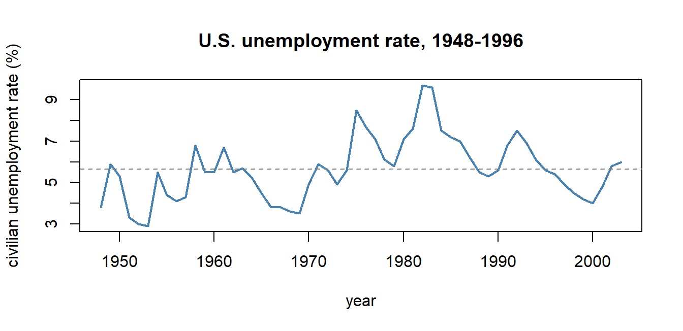
#| fig-cap: "A real macroeconomic time series: U.S. quarterly unemployment, 1948--1996 (Wooldridge `phillips` dataset). Notice that consecutive observations are obviously *not* independent draws from a population --- there are long expansions and long recessions, and a low unemployment year is almost always followed by another low year. That persistence is the same phenomenon we will call **autocorrelation** below. The cross-sectional ideal of MLR.2 (independent draws across $i$) cannot survive contact with data of this shape, and the rest of the chapter is about what to do about it."
#| fig-height: 3.4
library(wooldridge)
data("phillips")
plot(phillips$year, phillips$unem, type = "l", lwd = 2, col = "steelblue",
xlab = "year", ylab = "civilian unemployment rate (%)",
main = "U.S. unemployment rate, 1948-1996")
abline(h = mean(phillips$unem), lty = 2, col = "grey50")
```
Mechanically, almost everything from Chapters 2–6 carries over: OLS still solves $\min_{\beta} \sum_t (y_t - \mathbf{x}_t'\beta)^2$; the partialling-out interpretation is unchanged; nonlinear and qualitative regressors behave as before. What changes is the **error structure**. Two errors $u_t$ and $u_s$ refer to the *same* economic unit observed at *different* points in time, and there is no reason in general for them to be uncorrelated.
::: {.callout-note}
## Recap of MLR.2 (random sampling) in time-series context
Assumption MLR.2 in cross-sections required the sample to consist of $n$ *independent* draws --- for any pair $i\neq j$, $\mathbb{E}[u_i u_j]=0$. The mechanism that delivered MLR.2 was random sampling from a fixed population: knowing $u_i$ told you nothing about $u_j$.
In a time series there is no random sampling across units. Successive errors $u_t$ and $u_{t+1}$ are generated by the same process unfolding over time, and the natural default is that they *are* related. Whenever $\mathbb{E}[u_t u_s] \neq 0$ for some $t \neq s$, we say the errors are **autocorrelated** (or **serially correlated**). Will January's unobserved demand shock influence February's? Almost certainly yes --- that is the working definition of autocorrelation.
:::
The contrast with Chapter 7 is useful. Heteroskedasticity is a cross-sectional pathology in which $\operatorname{Var}(u_i)$ varies with the regressors but errors across units are independent. Autocorrelation is its time-series cousin: the off-diagonal elements of the error variance--covariance matrix are nonzero, while the diagonal may or may not stay constant. Both leave OLS unbiased but invalidate its standard errors.
## Definition, AR(1) structure, and consequences
### Definition
::: {.callout-note}
## Definition: autocorrelation
The errors $u_t$ exhibit **autocorrelation** (or **serial correlation**) when
$$
\operatorname{Cov}(u_t, u_s) \neq 0 \quad \text{for some } t \neq s.
$$
The variance--covariance matrix of $\mathbf{u} = (u_1,\dots,u_n)'$ is
$$
\operatorname{Var}(\mathbf{u}) =
\begin{pmatrix}
\sigma^2 & \gamma_1 & \gamma_2 & \cdots & \gamma_{n-1} \\
\gamma_1 & \sigma^2 & \gamma_1 & \cdots & \gamma_{n-2} \\
\gamma_2 & \gamma_1 & \sigma^2 & \cdots & \gamma_{n-3} \\
\vdots & \vdots & \vdots & \ddots & \vdots \\
\gamma_{n-1} & \gamma_{n-2} & \gamma_{n-3} & \cdots & \sigma^2
\end{pmatrix},
$$
with at least one off-diagonal element $\gamma_k = \operatorname{Cov}(u_t, u_{t-k}) \neq 0$.
:::
Under the classical cross-sectional assumptions, the off-diagonal entries are all zero and $\operatorname{Var}(\mathbf{u}) = \sigma^2 \mathbf{I}_n$. Autocorrelation drops that simplification.
### The AR(1) workhorse
Before any algebra, the picture. Think of $\rho$ as the fraction of yesterday's shock that carries over into today: if yesterday's error was $+2$ and $\rho = 0.7$, then today already starts with $1.4$ baked in before any new disturbance arrives. The closer $\rho$ is to $1$, the longer shocks live; at $\rho = 0$ each period is a fresh draw.
Almost all of the chapter --- and the vast majority of applied undergraduate work --- uses one specific model for serial dependence: the **first-order autoregressive** process, or AR(1):
$$
u_t = \rho\,u_{t-1} + \varepsilon_t, \qquad |\rho| < 1, \tag{AR(1)}
$$
where $\varepsilon_t$ is **white noise**: $\mathbb{E}[\varepsilon_t]=0$, $\operatorname{Var}(\varepsilon_t) = \sigma_\varepsilon^2$ constant, $\operatorname{Cov}(\varepsilon_t,\varepsilon_s)=0$ for $t \neq s$, and (often) $\varepsilon_t \sim \mathcal{N}(0,\sigma_\varepsilon^2)$.
The single parameter $\rho$ summarises the entire dependence structure. Under stationarity ($|\rho|<1$) one can show:
$$
\mathbb{E}[u_t] = 0, \qquad
\operatorname{Var}(u_t) = \frac{\sigma_\varepsilon^2}{1-\rho^2}, \qquad
\operatorname{Cov}(u_t, u_{t-k}) = \rho^k \cdot \frac{\sigma_\varepsilon^2}{1-\rho^2}.
$$
So $\gamma_k = \rho^k \sigma^2$ with $\sigma^2 = \sigma_\varepsilon^2/(1-\rho^2)$ --- the autocovariances **decay geometrically** in the lag $k$. The sign of $\rho$ classifies the pattern:
- **$\rho > 0$ (positive autocorrelation).** Errors of the same sign cluster. A positive shock today persists, decaying smoothly: long runs of positive residuals, then long runs of negative residuals. This is by far the most common case in macroeconomic and business data.
- **$\rho < 0$ (negative autocorrelation).** Errors alternate in sign: each positive shock is followed disproportionately by a negative one. Less common, but it does appear in inventory series and in models where adjustment overshoots.
- **$\rho = 0$ (no autocorrelation).** $u_t = \varepsilon_t$ and the errors are white noise: the cross-sectional default is restored.
```{r ch08-ar1-panel-fig}
#| echo: false
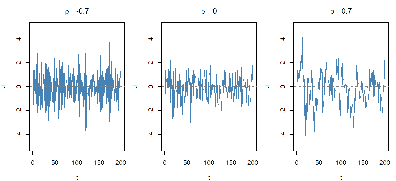
#| fig-cap: "Three simulated AR(1) error series of length 200, sharing the same innovation variance $\\sigma_\\varepsilon^2 = 1$ and the same random seed but different values of $\\rho$. Left ($\\rho = -0.7$): residuals alternate sign in a sawtooth pattern. Middle ($\\rho = 0$): white noise, no visible pattern. Right ($\\rho = 0.7$): long, smooth excursions above and below zero --- the cumulative-shock pattern of positive autocorrelation. Reading off the visual fingerprint is most of what graphical diagnostics do."
#| fig-height: 3.2
set.seed(42)
ar1_sim <- function(rho, n) {
u <- numeric(n); u[1] <- rnorm(1)
for (t in 2:n) u[t] <- rho * u[t - 1] + rnorm(1)
u
}
par(mfrow = c(1, 3), mar = c(4, 4, 3, 1))
for (rho_val in c(-0.7, 0, 0.7)) {
set.seed(42) # same seed for comparability across panels
series <- ar1_sim(rho_val, 200)
plot(seq_along(series), series, type = "l", lwd = 1.3, col = "steelblue",
xlab = "t", ylab = expression(u[t]),
main = bquote(rho == .(rho_val)),
ylim = c(-5, 5))
abline(h = 0, lty = 2, col = "grey50")
}
par(mfrow = c(1, 1))
```
Higher-order processes (AR(2), AR($p$), ARMA, …) exist and are studied in Econometrics II; for our purposes AR(1) is enough to fix ideas and to motivate the diagnostics and corrections that follow.
### Consequences for OLS
What does autocorrelation do to the OLS estimator $\hat{\beta}$?
1. **OLS is still unbiased and consistent** --- provided the conditional mean is correctly specified, i.e. $\mathbb{E}[u_t \mid \mathbf{x}_t] = 0$. Autocorrelation is a property of the *off-diagonal* elements of $\operatorname{Var}(\mathbf{u})$ and does not push the average estimate away from $\beta$. The point estimates are not the problem.
2. **OLS is no longer BLUE.** It is no longer the minimum-variance linear unbiased estimator; an alternative estimator (Generalised Least Squares, see §8.4) is more efficient.
3. **The conventional OLS standard errors are wrong.** The textbook formula $\operatorname{Var}(\hat{\beta}) = \sigma^2 (\mathbf{X}'\mathbf{X})^{-1}$ presupposes $\operatorname{Var}(\mathbf{u}) = \sigma^2 \mathbf{I}_n$, which fails. With **positive** autocorrelation the OLS-reported standard errors typically *understate* the true sampling variability, $t$-statistics are too large, $p$-values too small, and confidence intervals too narrow. The "optimistic $t$-statistics" of the motivating question are exactly this artefact.
::: {.callout-warning}
## Causality vs efficiency: the lagged-dependent-variable trap
There is one case in which autocorrelation does more than just inflate $t$-statistics: it destroys identification. If the regression includes a **lagged dependent variable** $y_{t-1}$ and the errors are AR(1),
$$
y_t = \alpha\,y_{t-1} + \beta_0 + \beta_1 x_t + u_t, \qquad u_t = \rho\,u_{t-1} + \varepsilon_t,
$$
then $y_{t-1}$ depends on $u_{t-1}$, and $u_{t-1}$ is correlated with $u_t$ through $\rho$. The regressor is correlated with the error, $\mathbb{E}[u_t \mid y_{t-1}] \neq 0$, and OLS is no longer just inefficient --- it becomes **biased and inconsistent**. The causal coefficient $\beta_1$ is no longer identified. This is the time-series cousin of the omitted-variable bias from Chapter 3.
:::
The intuition for why positive autocorrelation makes OLS standard errors too small is worth dwelling on: if successive errors carry information about one another, then $n$ correlated observations contain less independent information than $n$ uncorrelated ones. The effective sample size is smaller than the nominal $n$, but the OLS formula treats every observation as a fresh draw. The reported precision is therefore exaggerated.
## Detection
We have two complementary toolkits: *graphical* (quick, intuitive) and *analytical* (formal hypothesis tests). The recommended workflow is to look first and test second.
### Graphical methods
**Time plot of residuals.** Plot $\hat u_t$ against $t$. If the errors are uncorrelated, the residuals should scatter randomly around zero --- no visible pattern, no clustering, no obvious cycles. If you see **long runs** of same-sign residuals (many consecutive positives, then many consecutive negatives), that is the visual signature of $\rho>0$. If residuals alternate in a sawtooth pattern, that is $\rho<0$.
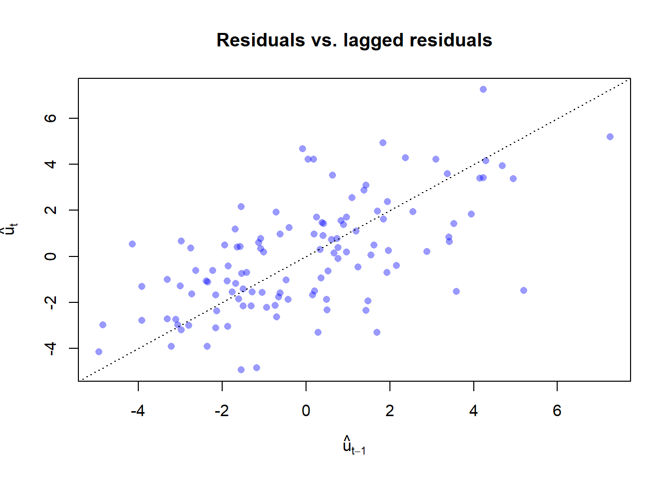
**Lag plot of residuals.** Plot $\hat u_t$ on the vertical axis against $\hat u_{t-1}$ on the horizontal axis. Under $\rho=0$ the cloud has no slope; under $\rho>0$ it tilts up-right (positive linear association); under $\rho<0$ it tilts down. Mechanically this is the picture of the OLS regression $\hat u_t = \rho\,\hat u_{t-1} + \text{(noise)}$, whose slope is exactly the estimate of $\rho$ that we will use below.
The three benchmark shapes are: a featureless cloud ($\rho\approx 0$), an upward-sloping line ($\rho>0$), and a downward-sloping line ($\rho<0$). In the lab below you will see all three.
### The Durbin–Watson test
The Durbin–Watson (DW) statistic is the workhorse formal test for first-order autocorrelation.
::: {.callout-note}
## Definition: Durbin–Watson statistic
$$
DW = \frac{\sum_{t=2}^{n} (\hat u_t - \hat u_{t-1})^2}{\sum_{t=1}^{n} \hat u_t^2}.
$$
The test is of $H_0: \rho = 0$ (no autocorrelation) against $H_1: \rho \neq 0$ (or a one-sided alternative).
:::
**Why $DW \approx 2(1-\hat\rho)$.** Expand the numerator:
$$
\sum_{t=2}^{n}(\hat u_t - \hat u_{t-1})^2
= \sum_{t=2}^{n} \hat u_t^2 \;-\; 2\sum_{t=2}^{n}\hat u_t \hat u_{t-1} \;+\; \sum_{t=2}^{n} \hat u_{t-1}^2.
$$
For large $n$ the two outer sums are each approximately $\sum_{t=1}^n \hat u_t^2$ (they differ by a single observation). Dividing through gives
$$
DW \;\approx\; \frac{2\sum_{t=2}^{n}\hat u_t^2 - 2\sum_{t=2}^{n} \hat u_t \hat u_{t-1}}{\sum_{t=1}^{n}\hat u_t^2}
\;=\; 2\left(1 - \frac{\sum_{t=2}^{n} \hat u_t \hat u_{t-1}}{\sum_{t=1}^{n}\hat u_t^2}\right)
\;=\; 2(1 - \hat\rho),
$$
where $\hat\rho = \sum_{t=2}^n \hat u_t \hat u_{t-1} \big/ \sum_{t=1}^n \hat u_t^2$ is the sample first-order autocorrelation of the residuals. Since $\rho\in[-1,1]$, the statistic lives in $[0,4]$:
- $DW \approx 0 \;\Leftrightarrow\; \hat\rho \approx +1$ (strong positive autocorrelation).
- $DW \approx 2 \;\Leftrightarrow\; \hat\rho \approx 0$ (no autocorrelation).
- $DW \approx 4 \;\Leftrightarrow\; \hat\rho \approx -1$ (strong negative autocorrelation).
**Bounds and decision rule.** The exact distribution of $DW$ depends on the design matrix $\mathbf{X}$, so Durbin and Watson tabulated a **lower bound** $d_L$ and an **upper bound** $d_U$ (functions of $n$, the number of regressors $k$, and the significance level). The decision rule, for the one-sided test $H_1:\rho>0$, is:
| Region | Conclusion |
|---------------------------------|---------------------------------------------|
| $0 < DW < d_L$ | Reject $H_0$: positive autocorrelation. |
| $d_L < DW < d_U$ | **Inconclusive.** |
| $d_U < DW < 4 - d_U$ | Do not reject $H_0$: no autocorrelation. |
| $4 - d_U < DW < 4 - d_L$ | **Inconclusive.** |
| $4 - d_L < DW < 4$ | Reject $H_0$: negative autocorrelation. |
```{r ch08-dw-numberline-fig}
#| echo: false
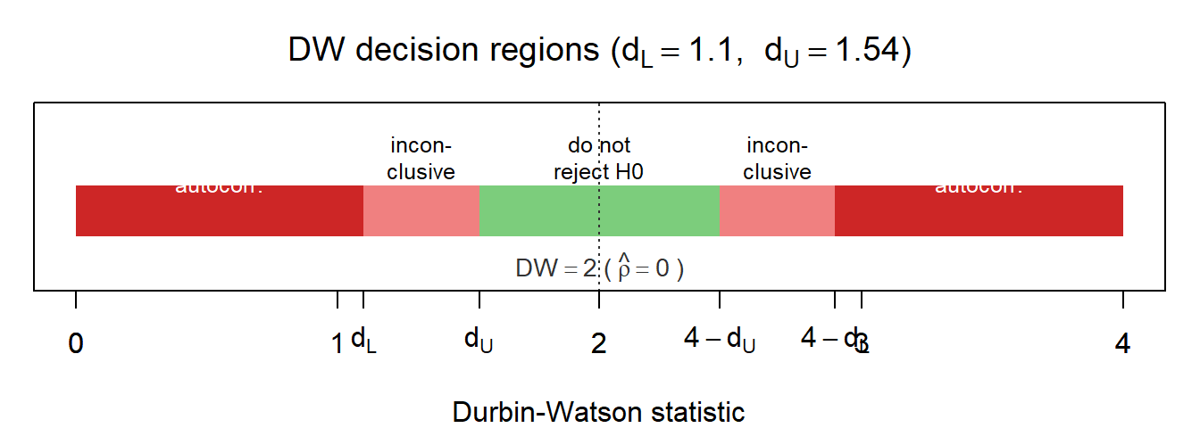
#| fig-cap: "The DW decision regions as a number line (illustrative bounds $d_L = 1.10$, $d_U = 1.54$, e.g. $n \\approx 30$, $k = 2$). The statistic lives in $[0, 4]$, with $DW = 2$ corresponding to $\\hat\\rho = 0$ (the dashed grey vertical). Red bands flag rejection; pink bands flag inconclusive regions; green flags 'no evidence against $H_0$'. Note the *symmetry*: positive autocorrelation pushes $DW$ down towards 0, negative autocorrelation pushes it up towards 4."
#| fig-height: 2.5
dL <- 1.10; dU <- 1.54
par(mar = c(4, 1, 3, 1))
plot(c(0, 4), c(0, 0), type = "n",
xlim = c(0, 4), ylim = c(-1.0, 1.4),
xlab = "Durbin-Watson statistic", ylab = "", yaxt = "n",
main = expression(paste("DW decision regions (",
d[L] == 1.10, ", ",
d[U] == 1.54, ")")))
rect(0, -0.35, dL, 0.35, col = "firebrick3", border = NA)
rect(dL, -0.35, dU, 0.35, col = "lightcoral", border = NA)
rect(dU, -0.35, 4 - dU, 0.35, col = "palegreen3", border = NA)
rect(4 - dU, -0.35, 4 - dL, 0.35, col = "lightcoral", border = NA)
rect(4 - dL, -0.35, 4, 0.35, col = "firebrick3", border = NA)
text(dL / 2, 0.75, "reject:\npositive\nautocorr.", cex = 0.78, col = "white")
text((dL + dU) / 2, 0.75, "incon-\nclusive", cex = 0.78)
text(2, 0.75, "do not\nreject H0", cex = 0.78)
text((4 - dU + 4 - dL) / 2, 0.75, "incon-\nclusive", cex = 0.78)
text((4 - dL + 4) / 2, 0.75, "reject:\nnegative\nautocorr.", cex = 0.78, col = "white")
abline(v = 2, lty = 3, col = "grey20")
text(2, -0.75, expression(DW == 2 ~ "(" ~ hat(rho) == 0 ~ ")"),
cex = 0.88, col = "grey20")
axis(1, at = c(0, dL, dU, 2, 4 - dU, 4 - dL, 4),
labels = c("0", expression(d[L]), expression(d[U]),
"2",
expression(4 - d[U]), expression(4 - d[L]),
"4"))
```
The two inconclusive regions are an unavoidable feature of the test --- a price one pays for not having to assume a particular design matrix. In modern software (e.g. `lmtest::dwtest()` in R) the test reports an exact $p$-value computed for the actual $\mathbf{X}$, sidestepping the table-bound mechanics. We use the bounds for hand exercises; we read the $p$-value in the lab.
::: {.callout-tip}
## Worked example (small-sample DW)
A regression of small road-accident counts $Y$ on registered cars $X$ over 10 years yields $\hat Y_t = 2.5676 + 0.04937\,X_t$ with $R^2 = 0.942$. From the table of residuals one computes
$$\sum_{t=2}^{n}(\hat u_t - \hat u_{t-1})^2 = 18.796,\quad \sum_{t=1}^{n}\hat u_t^2 = 22.844,$$
so
$$DW = \frac{18.796}{22.844} \approx 0.823.$$
For $n=10$ and $k=1$ regressors, the 5 % bounds are $d_L = 0.879$, $d_U = 1.320$. Since $DW < d_L$, we reject $H_0$ and conclude that the residuals exhibit **positive** first-order autocorrelation. (We will use this same example to illustrate Cochrane–Orcutt in §8.4.)
:::
### When DW fails: Durbin's $h$-test
The DW test rests on two assumptions that often go unstated: the error process is AR(1), and the regression does **not** include a lagged dependent variable. The lagged-dependent-variable case --- discussed in the warning box of §8.2.3 --- is precisely the case in which OLS becomes inconsistent, and where DW itself becomes badly biased toward 2 (toward the null of no autocorrelation), which is the worst possible behaviour for a diagnostic test.
For models of the form
$$
y_t = \alpha\,y_{t-1} + \beta_0 + \beta_1 x_{1t} + \cdots + \beta_k x_{kt} + u_t, \qquad u_t = \rho\,u_{t-1} + \varepsilon_t,
$$
Durbin proposed the **$h$ statistic**
$$
h \;=\; \hat\rho \,\sqrt{\frac{n}{1 - n\,\widehat{\operatorname{Var}}(\hat\alpha)}} \;\sim\; \mathcal{N}(0,1) \quad \text{under } H_0:\rho=0,
$$
where $\hat\alpha$ is the OLS coefficient on $y_{t-1}$ and $\widehat{\operatorname{Var}}(\hat\alpha)$ is the usual (incorrect) OLS variance estimate. One often plugs in $\hat\rho \approx 1 - DW/2$. Reject $H_0$ at level $\alpha$ if $|h| > z_{1-\alpha/2}$. If $n \cdot \widehat{\operatorname{Var}}(\hat\alpha) \geq 1$ the $h$ statistic is undefined (the radicand is non-positive); in that case use Breusch–Godfrey instead.
::: {.callout-tip}
## Worked example (Durbin's $h$)
Consider an OLS fit on $n=21$ observations:
$$\widehat Y_t = 1.3 + 0.97\,Y_{t-1} + 2.31\,X_t, \qquad \mathrm{se}(\hat\alpha) = 0.07, \qquad DW = 1.21.$$
Then $\hat\rho \approx 1 - 1.21/2 = 0.395$, $\widehat{\operatorname{Var}}(\hat\alpha) = 0.07^2 = 0.0049$, and
$$h = 0.395 \cdot \sqrt{\frac{21}{1 - 21 \cdot 0.0049}} = 0.395 \cdot 4.838 \approx 1.91.$$
At the 5 % level the critical value is $z_{0.975}=1.96$. Since $|h|=1.91 < 1.96$, we do **not** reject $H_0$: there is no statistically significant evidence of first-order autocorrelation. (A naive DW reading of $1.21$ might have suggested otherwise, but DW is biased here.)
:::
Other tests exist --- the Breusch–Godfrey LM test, which handles higher-order processes; the Ljung–Box portmanteau test on residual autocorrelations --- and are covered in Econometrics II. For this course, DW (or Durbin's $h$ when needed) is the standard tool.
## The robust shortcut: HAC standard errors
Before turning to a full correction, it is worth noting the time-series parallel of Chapter 7's robust standard errors. If all you want is honest standard errors and you don't care about the efficiency gain, **HAC** (Heteroskedasticity- and Autocorrelation-Consistent) standard errors are the one-line fix. They leave the OLS coefficients alone --- which, recall, are still unbiased under autocorrelation --- and just correct the variance, replacing the wrong $\sigma^2(\mathbf{X}'\mathbf{X})^{-1}$ with an estimator that accounts for the off-diagonal entries of $\operatorname{Var}(\mathbf{u})$. The Newey–West (1987) variance estimator is the standard implementation: it weights residual cross-products $\hat u_t \hat u_{t-k}$ by a kernel that down-weights distant lags, so the analyst does not have to commit to a specific error model like AR(1).
The trade-off is the same as for heteroskedasticity-robust SEs. HAC buys you valid inference under very weak assumptions, but it does not deliver an efficient estimator: with strong autocorrelation, GLS-style methods (next section) typically produce tighter confidence intervals. In modern applied work HAC is the default for time-series regressions where the error model is uncertain; Cochrane–Orcutt is reached for when one is willing to commit to AR(1) in exchange for efficiency. We show the modern one-line workflow first --- on a small simulated regression with AR(1) errors, paralleling the lab's full setup --- and then develop the GLS approach.
```{r ch08-hac-demo}
#| message: false
library(lmtest)
library(sandwich)

set.seed(1)
n_demo <- 100
x_demo <- 1:n_demo + rnorm(n_demo)
u_demo <- numeric(n_demo); u_demo[1] <- rnorm(1)
for (t in 2:n_demo) u_demo[t] <- 0.7 * u_demo[t-1] + rnorm(1)
y_demo <- 1 + 0.5 * x_demo + u_demo
fit_demo <- lm(y_demo ~ x_demo)

# OLS standard errors (wrong under autocorrelation):
coeftest(fit_demo)
# HAC (Newey-West) standard errors --- the one-line fix:
coeftest(fit_demo, vcov = NeweyWest(fit_demo))
```
The coefficients are identical in the two outputs --- HAC does not touch them --- but the standard errors in the second block are larger, the $t$-statistics smaller, and the $p$-values more honest. If you also want efficiency, read on for Cochrane–Orcutt.
## Correction: from GLS to Cochrane–Orcutt
If OLS is inefficient under AR(1), what should we do? The answer is **Generalised Least Squares (GLS)**: transform the model so that the transformed errors are white noise, then run OLS on the transformed model.
### The GLS quasi-difference
The trick: if today's error is part-yesterday's-error-plus-noise, then today minus $\rho$ times yesterday cancels out the dependence and leaves only the noise. That's the entire idea of GLS for AR(1).
Start from the model and its $\rho$-multiplied lag:
$$
y_t = \beta_0 + \beta_1 x_t + u_t, \qquad \rho\,y_{t-1} = \rho\beta_0 + \rho\beta_1 x_{t-1} + \rho\,u_{t-1}.
$$
Subtract the second from the first:
$$
y_t - \rho\,y_{t-1} = \beta_0(1-\rho) + \beta_1(x_t - \rho\,x_{t-1}) + (u_t - \rho\,u_{t-1}).
$$
By the AR(1) assumption $u_t - \rho\,u_{t-1} = \varepsilon_t$, which is white noise. Define the **quasi-differenced** variables
$$
y_t^* \;=\; y_t - \rho\,y_{t-1}, \qquad
x_t^* \;=\; x_t - \rho\,x_{t-1}, \qquad
\beta_0^{*} \;=\; \beta_0(1-\rho).
$$
The transformed regression
$$
y_t^* = \beta_0^* + \beta_1\,x_t^* + \varepsilon_t
$$
has homoskedastic, uncorrelated errors --- the classical regression assumptions are restored, and OLS on the transformed model is the **GLS estimator**, which is BLUE.
**The first observation.** The transformation as written loses observation $t=1$. To keep it, the **Prais–Winsten** modification rescales it differently:
$$
y_1^* = \sqrt{1-\rho^2}\,y_1, \qquad x_1^* = \sqrt{1-\rho^2}\,x_1, \qquad \text{constant}_1^* = \sqrt{1-\rho^2}.
$$
The factor $\sqrt{1-\rho^2}$ is exactly what makes $\operatorname{Var}(u_1^*) = \sigma_\varepsilon^2$, matching the other observations. In samples where $n$ is small, this matters; in large samples, dropping observation 1 (the "two-step Cochrane–Orcutt") is essentially equivalent.
In matrix form, the GLS transformation can be written compactly as
$$
\mathbf{Y}^* \;=\;
\begin{pmatrix}
\sqrt{1-\rho^2}\,y_1 \\
y_2 - \rho\,y_1 \\
\vdots \\
y_n - \rho\,y_{n-1}
\end{pmatrix},
\qquad
\mathbf{X}^* \;=\;
\begin{pmatrix}
\sqrt{1-\rho^2} & \sqrt{1-\rho^2}\,x_{21} & \cdots & \sqrt{1-\rho^2}\,x_{k1} \\
1-\rho & x_{22} - \rho\,x_{21} & \cdots & x_{k2} - \rho\,x_{k1} \\
\vdots & \vdots & \ddots & \vdots \\
1-\rho & x_{2n} - \rho\,x_{2,n-1} & \cdots & x_{kn} - \rho\,x_{k,n-1}
\end{pmatrix}.
$$
Running OLS on $(\mathbf{Y}^*, \mathbf{X}^*)$ delivers $\hat{\beta}_{\text{GLS}}$.
### The Cochrane–Orcutt iterative procedure
The catch: $\rho$ is unknown. We need to estimate it. The **Cochrane–Orcutt (CO)** procedure is the simplest feasible-GLS algorithm: alternate between estimating $\rho$ from residuals and re-estimating $\beta$ on the quasi-differenced data, until $\rho$ stabilises.
::: {.callout-note}
## Algorithm: Cochrane–Orcutt iterative procedure
1. Estimate the original model $y_t = \beta_0 + \beta_1 x_t + \cdots + u_t$ by OLS; collect residuals $\hat u_t$.
2. Estimate $\rho$ by regressing $\hat u_t$ on $\hat u_{t-1}$ (no intercept):
$$\hat\rho = \frac{\sum_{t=2}^{n}\hat u_t\,\hat u_{t-1}}{\sum_{t=2}^{n}\hat u_{t-1}^2}.$$
3. Form the quasi-differenced variables $y_t^* = y_t - \hat\rho\,y_{t-1}$, $x_t^* = x_t - \hat\rho\,x_{t-1}$ (and, if Prais–Winsten, the rescaled first observation).
4. Run OLS on $(y_t^*, x_t^*)$ to get new $\hat{\beta}^{(2)}$; compute new residuals $\hat u_t^{(2)}$.
5. Plug $\hat u_t^{(2)}$ back into step 2 to update $\hat\rho$.
6. Iterate until $\hat\rho$ converges (changes negligibly between iterations).
The final coefficient vector is the Cochrane–Orcutt FGLS estimate; reported standard errors are the OLS standard errors *from the transformed regression*, which are valid under AR(1).
:::
There are alternatives --- the two-step CO method (one iteration only), the Hildreth–Lu grid search over $\rho$, Durbin's two-step method, Prais–Winsten with restricted least squares --- but they all share the same underlying idea: estimate $\rho$, quasi-difference, and apply OLS to recover an efficient estimator.
::: {.callout-tip}
## Worked example (Cochrane–Orcutt on the accidents data)
Returning to the accidents-vs-cars example from §8.3.2: with $DW = 0.823$ and a small $n=10$, we apply the Prais–Winsten variant.
Step 1 (OLS): $\hat Y_t = 2.568 + 0.0494\,X_t$.
Step 2 ($\hat\rho$ from residuals): regressing $\hat u_t$ on $\hat u_{t-1}$ yields $\hat\rho = 0.4226$.
Step 3 (transform): for $t > 1$, $Y_t^* = Y_t - 0.4226\,Y_{t-1}$ and $X_t^* = X_t - 0.4226\,X_{t-1}$; for $t=1$, multiply by $\sqrt{1 - 0.4226^2} \approx 0.906$.
Step 4 (OLS on transformed): $\hat Y_t^* = 2.111 + 0.0498\,X_t^*$.
The slope barely moves --- OLS was unbiased to start with --- but the new DW computed on the transformed residuals is $1.52$, comfortably inside the no-autocorrelation region. The standard errors that come out of step 4 are the ones to report.
:::
The takeaway: in the AR(1) world, OLS gives you the right *point* estimates (on average) but the wrong *uncertainty*; Cochrane–Orcutt fixes the uncertainty without much changing the point.
## Lab: autocorrelation
The lab follows the workflow of Tutorial 9 (`autocorr_demo.xlsx`): regress quarterly sales on advertising and a time trend, diagnose autocorrelation visually and with Durbin–Watson, and correct it with Cochrane–Orcutt. To keep the chapter self-contained and reproducible without the external `.xlsx`, we generate a synthetic version of the tutorial dataset that has the same structure (sales depending on advertising and a trend, with AR(1) errors of known $\rho$). The interactive tutorial `LEARNR/08_autocorrelation.Rmd` uses an identical simulation.
```{r ch08-setup}
#| message: false
library(lmtest)
library(orcutt)

set.seed(2026)
n            <- 120                                    # quarterly observations, ~30 years
time         <- 1:n
advertising  <- 5 + 0.5 * time + rnorm(n, 0, 3)        # trending ad spend
rho_true     <- 0.7                                    # AR(1) parameter
u            <- numeric(n); u[1] <- rnorm(1, 0, 2)
for (t in 2:n) u[t] <- rho_true * u[t-1] + rnorm(1, 0, 2)
sales        <- 10 + 0.8 * advertising + 0.3 * time + u
autocorr_demo <- data.frame(time = time,
                            advertising = advertising,
                            sales = sales)
head(autocorr_demo)
```
The true data-generating process has slope `0.8` on advertising, a time-trend coefficient `0.3`, and AR(1) errors with $\rho = 0.7$ (strong positive autocorrelation). A real analyst would not know any of these numbers.
### OLS and a first look at the residuals
```{r ch08-ols}
fit <- lm(sales ~ advertising + time, data = autocorr_demo)
summary(fit)
```
The coefficient on `advertising` is in the right ballpark (around 0.8), the trend is in the right ballpark (around 0.3), and the $t$-statistics are spectacular. Are they real? Plot the residuals over time:
```{r ch08-residual-time}
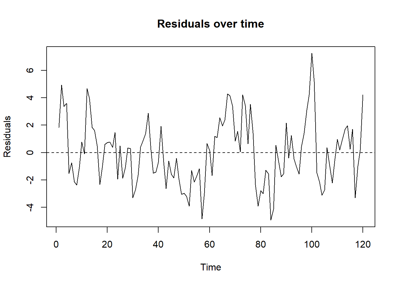
#| fig-cap: "OLS residuals plotted over time. Long runs of same-sign residuals are the visual signature of positive autocorrelation."
plot(ts(resid(fit)),
     ylab = "Residuals",
     main = "Residuals over time")
abline(h = 0, lty = 2)
```
The residuals trace out long, smooth excursions above and below zero: this is exactly the picture of $\rho>0$. Compare with what an uncorrelated residual series should look like (a featureless cloud around zero) and the difference is obvious.
### The lag plot
```{r ch08-lag-plot}
#| fig-cap: "Lag plot of OLS residuals: $\\hat u_t$ versus $\\hat u_{t-1}$. The upward tilt confirms positive first-order autocorrelation."
e <- resid(fit)
plot(head(e, -1), tail(e, -1),
     xlab = expression(hat(u)[t-1]),
     ylab = expression(hat(u)[t]),
     main = "Residuals vs. lagged residuals",
     pch  = 16,
     col  = rgb(0, 0, 1, 0.4))
abline(0, 1, lty = 3)
```
The slope of the cloud is the estimate of $\rho$. We can compute it directly:
```{r ch08-rho-from-residuals}
# Textbook sample autocorrelation, matching the algebra in section 8.3.2.
# An OLS slope of e on e_lag would be very close but not identical
# in finite samples; here we use the formula consistent with DW = 2(1 - rho_hat).
rho_hat <- sum(e[-1] * e[-n]) / sum(e^2)
rho_hat
2 * (1 - rho_hat) # back-of-envelope DW
```
The residual autocorrelation $\hat\rho$ should be close to the true $0.7$, and $2(1-\hat\rho)$ gives a quick approximation to what the Durbin–Watson statistic will report.
### Durbin–Watson
```{r ch08-dw}
dwtest(fit)
```
The DW statistic is well below 2, the $p$-value is tiny, and we reject $H_0: \rho = 0$ in favour of positive autocorrelation. (Compare DW to $2(1-\hat\rho)$ from the previous chunk: the two should agree to within rounding.)
### Cochrane–Orcutt correction
```{r ch08-co}
co <- cochrane.orcutt(fit)
summary(co)
```
`cochrane.orcutt()` iterates the algorithm of §8.4.2 until convergence and prints the corrected coefficients, the iterated $\hat\rho$, and a DW statistic computed on the transformed residuals.
::: {.callout-note}
## A note on `cochrane.orcutt()` vs Prais–Winsten
The algebra in §8.4.1 derived a Prais–Winsten transformation that *rescales* the first observation by $\sqrt{1 - \rho^2}$ so it can be retained. The `cochrane.orcutt()` function from the **orcutt** package implements the two-step Cochrane–Orcutt variant, which *drops* the first observation instead. With $n = 120$ as in our sample the two are essentially equivalent; in small samples the rescaling matters and you would want to use `prais::prais_winsten()` for a true Prais–Winsten fit. We stay with the dropped-first-observation variant here for compatibility with the §8.4.1 algorithm description.
:::
Compare the OLS and CO results side by side:
```{r ch08-compare}
cat("--- OLS coefficients ---\n")
print(round(coef(fit), 4))
cat("\n--- Cochrane-Orcutt coefficients ---\n")
print(round(co$coefficients, 4))
cat("\nEstimated rho:        ", round(co$rho, 4),
    "(true rho = ", rho_true, ")\n")
cat("DW after correction: ", round(co$DW[1], 4), "\n")
```
Two observations are typical of this kind of correction:
1. The **point estimates** of the slope coefficients barely move. OLS was unbiased, after all --- the only thing that was wrong with it was the uncertainty.
2. The **standard errors** in the CO output are larger than the OLS standard errors. The OLS $t$-statistics were inflated; the corrected ones are more honest. Hypotheses that were "highly significant" under OLS may become merely significant, or even fail to reject.
3. The DW statistic on the transformed residuals is close to 2, indicating that the AR(1) correction has done its job. (If it has not --- if DW is still far from 2 --- the residuals may follow a richer process such as AR(2), which is beyond the scope of this chapter.)
### A manual one-step Cochrane–Orcutt
To see exactly what `cochrane.orcutt()` does internally, here is a one-step version of the algorithm:
```{r ch08-manual-co}
y  <- autocorr_demo$sales
x1 <- autocorr_demo$advertising
x2 <- autocorr_demo$time

# Step 2: rho from residuals (already computed above as rho_hat)
# Step 3: quasi-differenced variables
y_q  <- y[-1]  - rho_hat * y[-n]
x1_q <- x1[-1] - rho_hat * x1[-n]
x2_q <- x2[-1] - rho_hat * x2[-n]

# Step 4: OLS on transformed model
fit_q <- lm(y_q ~ x1_q + x2_q)
summary(fit_q)$coefficients
# Recover the original-scale intercept
beta0_original_scale <- coef(fit_q)["(Intercept)"] / (1 - rho_hat)
beta0_original_scale
dwtest(fit_q) # DW should now be close to 2
```
One iteration already gets us most of the benefit. The fully iterated `cochrane.orcutt()` polishes $\hat\rho$ further until it converges; in practice a few iterations suffice.
::: {.callout-warning}
## Bias is not the worry --- uncertainty is
The OLS coefficient on `advertising` was unbiased, even with $\rho=0.7$ errors. The problem was that its standard error was *too small*. If you had taken the OLS $t$-statistic at face value and built a forecast confidence interval, your interval would have undercovered the truth --- exactly the cautionary tale of the motivating question.
A second cautionary tale belongs here too. If your residuals look autocorrelated, the *first* question is not "should I run Cochrane–Orcutt?" but "have I omitted a slowly-moving covariate that would explain the persistence?" Persistent residuals are sometimes a flag for missing controls --- a violation of MLR.4 that an AR(1) correction cannot fix. The "correlation is not causation" warning of Chapter 1 still applies in time series: HAC standard errors and Cochrane–Orcutt repair the inferential machinery, but they do not rescue a regression whose identifying assumption was wrong to begin with.
:::
## Self-check {.unnumbered}
Seven short multiple-choice questions. Try each one before opening the answer.
::: {.callout-tip collapse="true"}
## Q1. What autocorrelation is
Autocorrelation (serial correlation) means:
- A. $\operatorname{Var}(u_t)$ depends on the regressors $x_t$.
- B. $\operatorname{Cov}(u_t, u_s) \neq 0$ for some $t \neq s$ --- the errors are correlated across time periods.
- C. $x_t$ is correlated with $u_t$.
- D. $\mathbb{E}[u_t] \neq 0$.
**Answer: B.** Autocorrelation is a property of the *off-diagonal* elements of the error variance--covariance matrix. (A) is heteroskedasticity, (C) is endogeneity, (D) is a violation of zero-mean errors.
:::
::: {.callout-tip collapse="true"}
## Q2. Consequences for OLS
Under AR(1) errors but with $\mathbb{E}[u_t \mid x_t] = 0$, OLS is:
- A. Always biased.
- B. Always inconsistent.
- C. Still unbiased and consistent, but no longer BLUE, and the usual standard errors are wrong.
- D. Still BLUE.
**Answer: C.** OLS keeps its point-estimate properties but loses efficiency and produces invalid standard errors. (B) becomes correct only in the special case of a lagged dependent variable.
:::
::: {.callout-tip collapse="true"}
## Q3. The AR(1) process
In the model $u_t = \rho u_{t-1} + \varepsilon_t$ with $|\rho|<1$ and $\varepsilon_t$ white noise, autocorrelation is:
- A. Positive when $\rho > 0$, negative when $\rho<0$; the autocovariances decay geometrically.
- B. Always positive.
- C. Independent of $\rho$.
- D. Equivalent to heteroskedasticity.
**Answer: A.** The sign of $\rho$ pins down the pattern, and $\operatorname{Cov}(u_t, u_{t-k}) = \rho^k \sigma^2$ decays geometrically with the lag.
:::
::: {.callout-tip collapse="true"}
## Q4. Reading the residual time plot
A plot of OLS residuals against time shows long runs of positive residuals followed by long runs of negative residuals. This suggests:
- A. Positive autocorrelation.
- B. Negative autocorrelation.
- C. Heteroskedasticity.
- D. No systematic pattern.
**Answer: A.** Persistent same-sign runs are the visual signature of $\rho>0$. Sawtooth patterns (alternating signs) suggest $\rho<0$.
:::
::: {.callout-tip collapse="true"}
## Q5. The DW statistic
The Durbin–Watson statistic satisfies, for large $n$:
- A. $DW = \hat\rho$.
- B. $DW = 1 + \hat\rho$.
- C. $DW \approx 2(1 - \hat\rho)$.
- D. $DW = 2\hat\rho$.
**Answer: C.** Expanding the squared differences in the numerator and using $\sum \hat u_t^2 \approx \sum \hat u_{t-1}^2$ for large $n$ gives $DW \approx 2(1-\hat\rho)$.
:::
::: {.callout-tip collapse="true"}
## Q6. When DW is not valid
The Durbin–Watson test is **not** valid when:
- A. The errors are normally distributed.
- B. The sample size is large.
- C. There are many regressors.
- D. The model includes a lagged dependent variable.
**Answer: D.** A lagged dependent variable creates correlation between regressor and error, biases DW toward 2, and ruins the test. Use Durbin's $h$ instead.
:::
::: {.callout-tip collapse="true"}
## Q7. After Cochrane–Orcutt
After a successful Cochrane–Orcutt correction, the DW statistic computed on the transformed regression should:
- A. Be close to 0.
- B. Be close to 4.
- C. Equal $\hat\rho$.
- D. Be close to 2.
**Answer: D.** A successful AR(1) correction whitens the residuals, so $\hat\rho^*$ on the transformed model is close to 0 and $DW^* \approx 2(1-0) = 2$. If DW after correction is still far from 2, the AR(1) assumption is wrong.
:::
The fuller interactive set (twelve items including simulation exercises) lives in `LEARNR/08_autocorrelation.Rmd`.
## Exercises {.unnumbered}
**Exercise 8.1 ★ --- Reading a Durbin–Watson statistic.** A regression of quarterly retail sales on advertising spending and a time trend uses $n=80$ quarters and $k=2$ regressors. The OLS output reports $DW = 0.94$. The relevant 5 % bounds are $d_L = 1.59$, $d_U = 1.69$. State your conclusion and explain what it implies for the OLS $t$-statistics in the regression.
::: {.callout-tip collapse="true"}
## Show answer
Since $0 < DW < d_L$ (i.e. $0.94 < 1.59$), we reject $H_0:\rho=0$ in favour of $H_1:\rho>0$: there is positive first-order autocorrelation. The implied $\hat\rho \approx 1 - DW/2 = 0.53$. The OLS standard errors are therefore too small, the $t$-statistics inflated, and any "significant" coefficients should be re-tested using Cochrane–Orcutt or a Newey–West HAC variance estimator.
:::
**Exercise 8.2 ★ --- Sign of autocorrelation from a lag plot.** A scatter of $\hat u_t$ against $\hat u_{t-1}$ shows a clear *downward*-sloping cloud, with most points in the upper-left and lower-right quadrants. What is the approximate sign of $\rho$? What would the DW statistic be approximately?
::: {.callout-tip collapse="true"}
## Show answer
Downward slope $\Rightarrow \hat\rho < 0$: **negative** autocorrelation. With (say) $\hat\rho \approx -0.5$ we have $DW \approx 2(1 - (-0.5)) = 3$, comfortably above 2.
:::
**Exercise 8.3 ★★ --- DW from a residual table.** Using the small-sample example of §8.3.2, $\sum_{t=2}^{n}(\hat u_t - \hat u_{t-1})^2 = 18.796$ and $\sum_{t=1}^{n}\hat u_t^2 = 22.844$.
(a) Compute the DW statistic and the implied $\hat\rho$.
(b) For $n=10$, $k=1$, the 5 % bounds are $d_L = 0.879$, $d_U = 1.320$. What do you conclude?
(c) Briefly explain why the bounds depend on $n$ and $k$.
::: {.callout-tip collapse="true"}
## Show answer
(a) $DW = 18.796/22.844 \approx 0.823$, so $\hat\rho \approx 1 - DW/2 \approx 0.589$. (b) Since $DW < d_L$, reject $H_0$: positive autocorrelation. (c) The exact distribution of $DW$ depends on $\mathbf{X}'\mathbf{X}$; Durbin and Watson bracketed it with two bounds that depend only on $(n,k)$, leaving an inconclusive region.
:::
**Exercise 8.4 ★★ --- Durbin's $h$.** An OLS regression with $n=21$ produces
$$\widehat Y_t = 1.3 + 0.97\,Y_{t-1} + 2.31\,X_t, \qquad \mathrm{se}(\hat\alpha)=0.07,\qquad DW = 1.21.$$
Compute Durbin's $h$ statistic and decide whether the residuals are autocorrelated at the 5 % level. Why is $DW$ alone misleading here?
::: {.callout-tip collapse="true"}
## Show answer
$\hat\rho \approx 1 - 1.21/2 = 0.395$; $\widehat{\operatorname{Var}}(\hat\alpha) = 0.07^2 = 0.0049$;
$$h = 0.395 \sqrt{21/(1 - 21\cdot 0.0049)} \approx 1.91.$$
Critical value $z_{0.975}=1.96$; $|h|<1.96$, do **not** reject $H_0$. The plain DW reading of 1.21 is biased toward 2 (the null) because the regression contains $Y_{t-1}$; trusting DW would have falsely flagged autocorrelation.
:::
**Exercise 8.5 ★★ --- Why positive autocorrelation deflates OLS standard errors (sketch).** In one short paragraph, explain --- using the idea of *effective sample size* --- why positive serial correlation makes the conventional OLS standard error of $\hat\beta_1$ in $y_t = \beta_0 + \beta_1 x_t + u_t$ too small. You do not need to derive a formula; an intuition based on the information content of $n$ correlated observations is enough.
*A full answer is given in the Instructor Edition.*
**Exercise 8.6 ★★★ --- One-step Cochrane–Orcutt by hand.** A small dataset has $\hat\rho = 0.4226$ obtained from the OLS residuals of $Y_t = \beta_0 + \beta_1 X_t + u_t$ on $n=10$ observations.
(a) Write down the formulas for the quasi-differenced variables $Y_t^*$, $X_t^*$ and the transformed constant term, *including* the Prais–Winsten treatment of $t=1$.
(b) Explain why the standard error of $\hat\beta_1$ computed on $(Y_t^*, X_t^*)$ is the one to report, while the OLS standard error from the *original* regression is not.
(c) After running OLS on $(Y_t^*, X_t^*)$ the new $DW$ statistic is $1.52$. With $n=9$, $k=1$, $d_L=0.824$, $d_U=1.320$, would you iterate again or stop?
*A full answer is given in the Instructor Edition.*