Appendix A — Mathematical and Statistical Prerequisites
This appendix collects the mathematical and statistical tools used throughout the book. It is meant as a reference: skim it once at the start of the course, then come back to individual sections as they are invoked. The level is deliberately operational — enough to follow the derivations in the main text without turning the book into a course on real analysis (Wooldridge 2020). We adopt Wooldridge’s notation everywhere: population parameters are \(\beta_0, \beta_1, \dots\); the population error is \(u\); the sample residual is \(\hat u\); fitted values are \(\hat y\); and the usual sums of squares are SST, SSE, and SSR.
Learning outcomes
By the end of this appendix the reader should be able to:
- Manipulate exponents and logarithms confidently, and read off elasticities and semi-elasticities from log-transformed equations.
- Compute single-variable derivatives and partial derivatives, and use first-order conditions to solve a small optimisation problem.
- State and apply the linearity of expectation, the formulas for variance and covariance, and the conditional-expectation properties used by Wooldridge.
- Recall the shapes and uses of the normal, \(t\), \(\chi^2\), and \(F\) distributions, and locate critical values in standard tables.
- Read and manipulate a vector or matrix, including transpose, inverse, and rank, well enough to follow the matrix form of OLS in §3.4.
- Install R and RStudio, load the
wooldridgepackage, and run a first inspection of thewage1dataset.
A.1 A.1 Algebra refresher
A.1.1 Functions and notation
A function \(f: \mathbb{R} \to \mathbb{R}\) assigns to each real number \(x\) a real number \(f(x)\). The graphs we draw in this book are almost always of functions of one or two variables. A linear function takes the form
\[ f(x) = \beta_0 + \beta_1 x, \]
with intercept \(\beta_0\) and slope \(\beta_1\). The slope \(\beta_1\) tells us by how many units \(f(x)\) changes when \(x\) increases by one unit. This is exactly how we will read every estimated coefficient in the book.
A.1.2 Exponents and powers
Every interest-rate, growth, and elasticity calculation you will do this term either is an exponentiation or hides one inside exp(...) or log(...), so the rules below are the algebraic plumbing of the entire course.
For any \(a > 0\) and any real numbers \(m, n\):
\[ a^{m} \cdot a^{n} = a^{m+n},\qquad \frac{a^{m}}{a^{n}} = a^{m-n},\qquad (a^{m})^{n} = a^{mn},\qquad a^{0} = 1. \]
(The same identities hold for any real \(a \neq 0\) when \(m, n\) are integers; the \(a > 0\) restriction matters as soon as we allow fractional exponents — for instance, the square root, \(\sqrt{a} = a^{1/2}\), is defined for \(a \geq 0\) only.)
A.1.3 Logarithms
Logging a regressor lets us read coefficients as percentage effects, which is half of what makes regressions communicable to non-economists — so the log rules below are not optional.
The natural logarithm \(\ln(x)\) is the inverse of the exponential function \(e^{x}\): \(\ln(e^{x}) = x\) and \(e^{\ln(x)} = x\) for \(x > 0\). The properties we use over and over are:
\[ \ln(xy) = \ln(x) + \ln(y),\quad \ln\!\left(\tfrac{x}{y}\right) = \ln(x) - \ln(y),\quad \ln(x^{a}) = a\,\ln(x),\quad \ln(1) = 0. \]
A useful approximation, exploited throughout the book, is that for small changes,
\[ \ln(x + \Delta x) - \ln(x) \approx \frac{\Delta x}{x}. \]
That is, a difference of logs is approximately a percentage change. This is why log-transformed regressions are so popular in applied work — they let us read coefficients as elasticities or percentage effects.
NoteDefinition: elasticity and semi-elasticity
In the log-log specification \(\ln(y) = \beta_0 + \beta_1 \ln(x) + u\), the coefficient \(\beta_1\) is an elasticity: a 1% increase in \(x\) raises \(y\) by approximately \(\beta_1\)%.
In the log-level specification \(\ln(y) = \beta_0 + \beta_1 x + u\), the coefficient \(\beta_1\) is a semi-elasticity: a one-unit increase in \(x\) raises \(y\) by approximately \(100\,\beta_1\%\).
Forward reference: these interpretations are used systematically from Chapter 2 onwards, and become central in the dummy-variables chapter where we read \(\beta_1\) as a “log-wage gap” of \(100\,\beta_1\)%.
A.1.4 Summations
Every estimator in the book is a sum — \(\hat\beta_1\), \(\bar y\), \(\mathrm{SST}_x\) — so once you can manipulate \(\sum\) cleanly, you can manipulate OLS.
The summation symbol \(\sum\) is shorthand we cannot live without:
\[ \sum_{i=1}^{n} x_i = x_1 + x_2 + \cdots + x_n. \]
Two properties used constantly:
\[ \sum_{i=1}^{n} (a x_i + b y_i) = a \sum_{i=1}^{n} x_i + b \sum_{i=1}^{n} y_i,\qquad \sum_{i=1}^{n} c = n\,c. \]
The sample mean is \(\bar x = \tfrac{1}{n}\sum_{i=1}^{n} x_i\), and a property we will use in the OLS derivation is \(\sum_{i=1}^{n} (x_i - \bar x) = 0\).
WarningCommon mistake: \(\ln(x + y) \ne \ln(x) + \ln(y)\)
The log of a sum is not the sum of the logs. This trips up many first-time users when they try to “simplify” terms like \(\ln(\beta_0 + \beta_1 x)\) — they cannot be split. Logarithms split products, not sums.
A.2 A.2 Calculus refresher
A.2.1 Derivatives of a single variable
OLS is the algorithm that sets the derivative of the sum of squared residuals to zero; you cannot derive a single coefficient in this book without this tool.
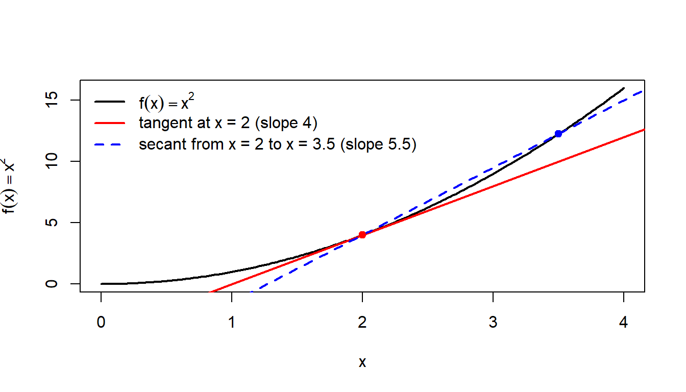
The derivative \(f'(x)\) measures the instantaneous rate of change of \(f\) at \(x\):
\[ f'(x) = \lim_{h \to 0} \frac{f(x + h) - f(x)}{h}. \]
Visually, the derivative is the slope of the tangent to the graph of \(f\) at \(x\). The fraction inside the limit is the slope of a secant between two nearby points \(x\) and \(x + h\); as \(h\) shrinks, the secant pivots towards the tangent.
The rules we need are short:
\[ \frac{d}{dx}(c) = 0,\quad \frac{d}{dx}(x^{n}) = n\,x^{n-1},\quad \frac{d}{dx}\!\left(e^{x}\right) = e^{x},\quad \frac{d}{dx}\!\left(\ln x\right) = \frac{1}{x}. \]
Linearity, product, quotient, and chain rules:
\[ (af + bg)' = a f' + b g',\qquad (fg)' = f'g + fg', \] \[ \left(\frac{f}{g}\right)' = \frac{f'g - fg'}{g^{2}},\qquad (f\circ g)'(x) = f'\!\bigl(g(x)\bigr)\, g'(x). \]
A.2.2 Partial derivatives
This is the ceteris paribus interpretation of \(\beta_j\): the partial derivative of \(\mathbb{E}[y \mid \mathbf{x}]\) with respect to \(x_j\), holding the other regressors fixed. Everything Chapter 3 says about “controlling for” is the operator below in disguise.
For a function of several variables \(f(x_1, x_2, \dots, x_k)\), the partial derivative with respect to \(x_j\) holds the other variables fixed:
\[ \frac{\partial f}{\partial x_j} = \lim_{h\to 0} \frac{f(\dots, x_j + h, \dots) - f(\dots, x_j, \dots)}{h}. \]
This is precisely the ceteris paribus reading we want from a multiple regression: for the population model
\[ y = \beta_0 + \beta_1 x_1 + \beta_2 x_2 + u, \]
we have \(\partial y / \partial x_1 = \beta_1\) holding \(x_2\) fixed — the so-called partial effect. Chapter 3 makes this interpretation precise.
A.2.3 First-order conditions and optimisation
Both OLS (minimising SSR) and Maximum Likelihood (maximising the log-likelihood) reduce to the same three-step recipe: take derivatives, set them to zero, solve.
To find an interior minimum or maximum of a smooth function, set the derivative to zero (the first-order condition, FOC) and check the second-order condition. A sufficient condition for a strict local minimum is \(f''(x^\star) > 0\); the necessary second-order condition is the weaker \(f''(x^\star) \geq 0\). The distinction matters because edge cases like \(f(x) = x^4\) have a minimum at \(x = 0\) with \(f''(0) = 0\). For functions of several variables, set every partial derivative to zero simultaneously.
NoteExample: minimising a simple quadratic
Consider \(f(\beta) = \sum_{i=1}^{n} (y_i - \beta)^{2}\). The FOC is
\[ \frac{d f}{d \beta} = -2\sum_{i=1}^{n} (y_i - \beta) = 0 \;\Longleftrightarrow\; \beta = \frac{1}{n}\sum_{i=1}^{n} y_i = \bar y. \]
The minimiser is the sample mean. This is exactly the structure of OLS: OLS minimises a sum of squared residuals by setting partial derivatives equal to zero. We carry out this derivation in detail in §2.4.
A.3 A.3 Probability refresher
A.3.1 Random variables
A random variable \(X\) is a numerical summary of the outcome of a random experiment. It is discrete if it can take only a countable number of values (e.g. the number of children in a household), and continuous if it can take any value in an interval (e.g. an hourly wage). Throughout the book we write the (unknown) population mean as \(\mu = \mathbb{E}[X]\) and the population variance as \(\sigma^{2} = \operatorname{Var}(X)\).
A.3.2 Expectation
The expected value of \(X\), denoted \(\mathbb{E}[X]\), is a population average. The properties below are used on essentially every page of the book.
\[ \mathbb{E}[c] = c,\qquad \mathbb{E}[aX + b] = a\,\mathbb{E}[X] + b, \] \[ \mathbb{E}[aX_1 + bX_2] = a\,\mathbb{E}[X_1] + b\,\mathbb{E}[X_2],\qquad \mathbb{E}\!\left[\sum_{i=1}^{n} a_i X_i\right] = \sum_{i=1}^{n} a_i\,\mathbb{E}[X_i]. \]
The last identity is linearity of expectation: it holds whether or not the \(X_i\) are independent.
A.3.3 Variance
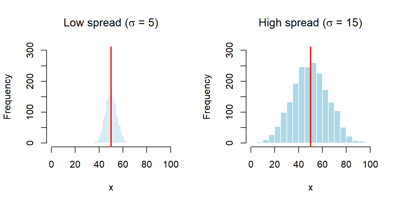
The variance measures dispersion around the mean:
\[ \operatorname{Var}(X) = \sigma^{2} = \mathbb{E}\!\bigl[(X - \mathbb{E}[X])^{2}\bigr] = \mathbb{E}[X^{2}] - \bigl(\mathbb{E}[X]\bigr)^{2}. \]
The standard deviation is \(\sigma = \sqrt{\operatorname{Var}(X)}\) and has the same units as \(X\). Useful properties:
\[ \operatorname{Var}(c) = 0,\qquad \operatorname{Var}(aX + b) = a^{2}\operatorname{Var}(X). \]
Notice that an additive constant \(b\) shifts the distribution but does not affect its dispersion. A multiplicative constant \(a\) scales the variance by \(a^{2}\), not by \(a\).
A.3.4 Covariance and correlation
The covariance between two random variables measures the direction of their linear co-movement:
\[ \operatorname{Cov}(X, Y) = \mathbb{E}\!\bigl[(X - \mathbb{E}[X])(Y - \mathbb{E}[Y])\bigr] = \mathbb{E}[XY] - \mathbb{E}[X]\,\mathbb{E}[Y]. \]
If either \(\mathbb{E}[X] = 0\) or \(\mathbb{E}[Y] = 0\), the second expression collapses to \(\operatorname{Cov}(X, Y) = \mathbb{E}[XY]\). Properties:
\[ \operatorname{Cov}(aX, bY) = ab\,\operatorname{Cov}(X, Y),\qquad \operatorname{Cov}(X, X) = \operatorname{Var}(X). \]
If \(X\) and \(Y\) are independent, then \(\operatorname{Cov}(X, Y) = 0\). The converse is false in general: zero covariance only rules out linear dependence. The correlation coefficient rescales the covariance to lie in \([-1, 1]\):
\[ \operatorname{Corr}(X, Y) = \rho_{XY} = \frac{\operatorname{Cov}(X, Y)}{\sqrt{\operatorname{Var}(X)}\sqrt{\operatorname{Var}(Y)}}. \]
A.3.5 Variance of a sum
A formula we will use many times in the book is
\[ \operatorname{Var}(aX + bY) = a^{2}\operatorname{Var}(X) + b^{2}\operatorname{Var}(Y) + 2ab\,\operatorname{Cov}(X, Y). \]
When \(\operatorname{Cov}(X, Y) = 0\) this simplifies to \(\operatorname{Var}(X + Y) = \operatorname{Var}(X) + \operatorname{Var}(Y)\). The general \(n\)-variable version,
\[ \operatorname{Var}\!\left(\sum_{i=1}^{n} a_i X_i\right) = \sum_{i=1}^{n} a_i^{2}\,\operatorname{Var}(X_i) + 2\sum_{i<j} a_i a_j\,\operatorname{Cov}(X_i, X_j), \]
is invoked when we derive the sampling variance of the OLS estimator.
A.3.6 Conditional expectation
The conditional expectation \(\mathbb{E}[Y \mid X]\) is the mean of \(Y\) given knowledge of \(X\). It is itself a function of \(X\). The properties we use most often are:
\[ \mathbb{E}[X \mid X] = X,\qquad \mathbb{E}\bigl[g(X) \mid X\bigr] = g(X), \] \[ \mathbb{E}\bigl[a Y + b(X) \mid X\bigr] = a\,\mathbb{E}[Y \mid X] + b(X). \]
If \(X\) and \(Y\) are independent, \(\mathbb{E}[Y \mid X] = \mathbb{E}[Y]\). Finally, the Law of Iterated Expectations (also called the tower property) is the single most useful tool in the book:
\[ \mathbb{E}\bigl[\mathbb{E}[Y \mid X]\bigr] = \mathbb{E}[Y]. \]
The zero conditional mean assumption \(\mathbb{E}[u \mid x] = 0\) that underpins OLS unbiasedness in §3.2 is a statement about conditional expectation in exactly this sense.
WarningCommon mistake: \(\operatorname{Cov}(X, Y) = 0\) does not mean independence
Zero covariance only rules out linear association. Two variables can have \(\operatorname{Cov}(X, Y) = 0\) and still be deterministically related — the textbook example is \(X \sim \text{Uniform}(-1, 1)\) and \(Y = X^{2}\), which satisfy \(\operatorname{Cov}(X, Y) = 0\) even though \(Y\) is a function of \(X\).
A.4 A.4 Statistical inference refresher
A.4.1 Sampling distributions
We will repeatedly contrast a population quantity (e.g. \(\beta_1\)) with its estimator computed from a sample (e.g. \(\hat \beta_1\)). The estimator is itself a random variable — it varies from sample to sample — and its distribution is called the sampling distribution. Two features of the sampling distribution determine the quality of the estimator:
- The mean: an estimator \(\hat\theta\) is unbiased for \(\theta\) if \(\mathbb{E}[\hat\theta] = \theta\).
- The variance: among linear unbiased estimators, the one with the smallest variance is the most efficient. The Gauss-Markov theorem in Chapter 3 makes this comparison formal for OLS. The “linear” qualifier is load-bearing: nonlinear estimators (ridge, LASSO, quantile regression) can sometimes do strictly better in mean-squared-error terms by accepting a small bias in exchange for a large variance reduction.
A.4.2 The Central Limit Theorem
If \(X_1, X_2, \dots, X_n\) are independent and identically distributed (i.i.d.) with mean \(\mu\) and variance \(\sigma^{2} < \infty\), then
\[ \sqrt{n}\,\frac{\bar X_n - \mu}{\sigma} \;\xrightarrow{d}\; \mathcal{N}(0, 1)\quad\text{as } n \to \infty. \]
The remarkable point is that the shape of the underlying distribution of \(X_i\) does not matter: the sample mean is approximately normal in large samples, whatever \(X\) looks like. This is why \(t\)- and \(z\)-statistics built from OLS estimators are approximately normal in large samples, even when the errors \(u\) are not.
A.4.3 The normal distribution
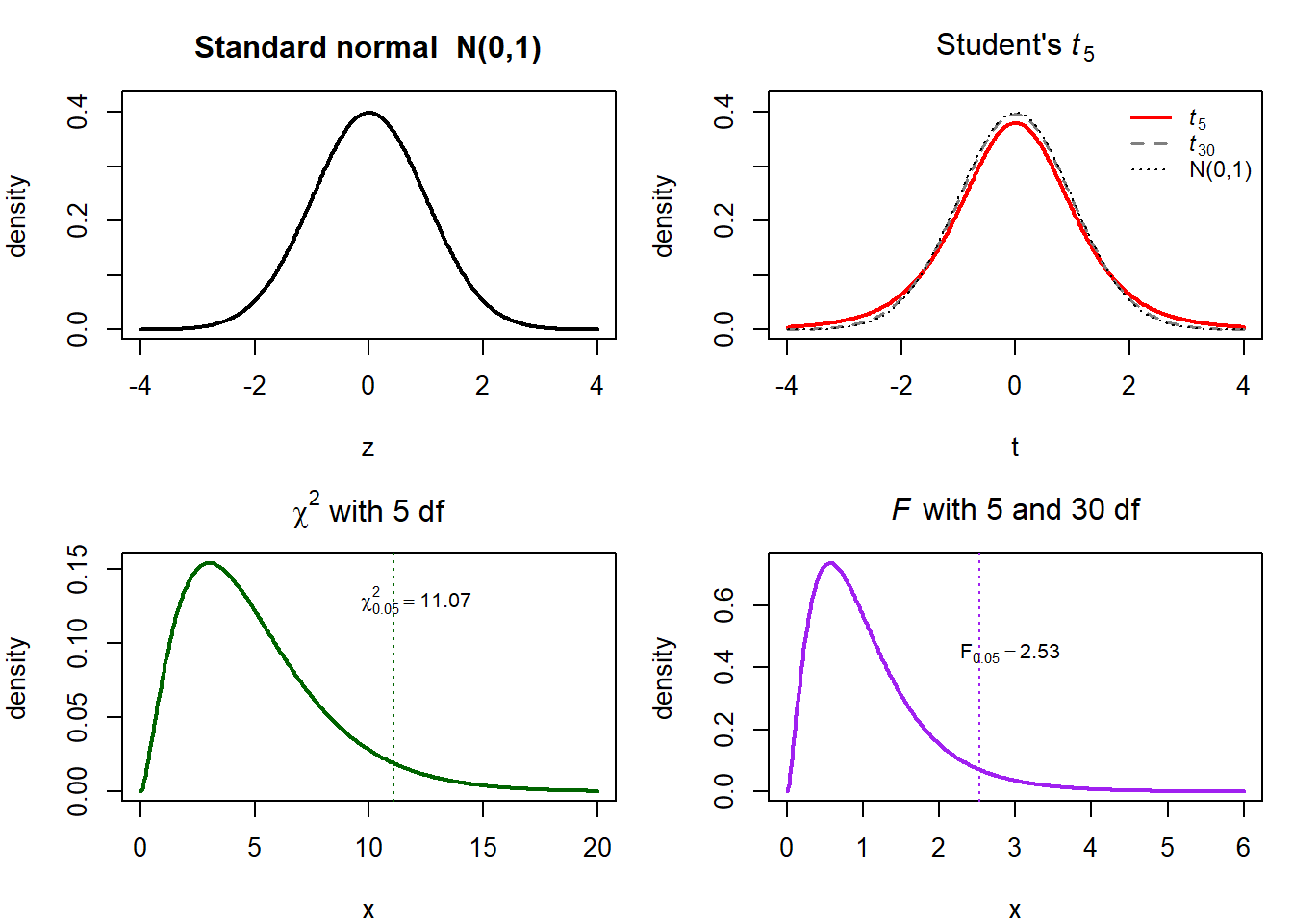
The standard normal \(\mathcal{N}(0, 1)\) has density
\[ \phi(z) = \frac{1}{\sqrt{2\pi}}\,\exp\!\left(-\tfrac{1}{2} z^{2}\right), \]
is symmetric about \(0\), and has \(\mathbb{E}[Z] = 0\), \(\operatorname{Var}(Z) = 1\). Two-sided critical values you will memorise: \(z_{0.975} = 1.96\) (5% level) and \(z_{0.995} = 2.576\) (1% level). A general normal \(X \sim \mathcal{N}(\mu, \sigma^{2})\) can always be standardised to \(Z = (X - \mu)/\sigma\).
A.4.4 The \(t\), \(\chi^{2}\), and \(F\) distributions
These three distributions appear naturally when we test hypotheses about regression coefficients.
- The \(\chi^{2}_{k}\) distribution is the distribution of a sum of \(k\) squared independent standard normals. It is non-negative, right-skewed, and has mean \(k\).
- The \(t_{k}\) distribution is the ratio \(Z / \sqrt{V/k}\) where \(Z \sim \mathcal{N}(0, 1)\) and \(V \sim \chi^{2}_{k}\) are independent. It is symmetric and bell-shaped, with heavier tails than the standard normal; as \(k\to\infty\) it converges to \(\mathcal{N}(0, 1)\).
- The \(F_{k_1, k_2}\) distribution is the ratio \((V_1/k_1) / (V_2/k_2)\) of two independent \(\chi^{2}\) random variables divided by their respective degrees of freedom. It is non-negative and right-skewed.
In §4.3 we will use \(t\)-statistics for single-coefficient tests, \(F\)-statistics for joint tests, and \(\chi^{2}\) variants for large-sample tests. Critical values are tabulated in any statistical software; in R you will use qt(), qf(), and qchisq().
NoteDefinition: \(p\)-value
The \(p\)-value of a test is the probability, under the null hypothesis, of observing a test statistic at least as extreme as the one we got. Small \(p\)-values are evidence against the null. The conventional thresholds are 1%, 5%, and 10%, but the \(p\)-value itself is what you should report — not just “rejected” or “not rejected”.
A.4.5 Confidence intervals
A \((1 - \alpha)\) confidence interval for a parameter \(\theta\) is a random interval that, in repeated samples, contains the true \(\theta\) with probability \(1 - \alpha\). For an estimator \(\hat\theta\) with approximate normal sampling distribution and standard error \(\mathrm{se}(\hat\theta)\), the standard 95% interval is \(\hat\theta \pm 1.96 \cdot \mathrm{se}(\hat\theta)\). Chapter 4 builds confidence intervals for individual OLS coefficients in exactly this form.
A.5 A.5 Linear algebra refresher
The matrix form of OLS in §3.4 needs a small bag of linear-algebra tools. We collect them here.
A.5.1 Vectors and matrices
Wooldridge writes the multiple-regression model as \(\mathbf{y} = \mathbf{X}\beta + \mathbf{u}\), and the rest of his Chapter 3 is one long matrix calculation — you need to be able to follow it.
A column vector of length \(n\) is a stack of \(n\) real numbers:
\[ \mathbf{x} = \begin{pmatrix} x_1 \\ x_2 \\ \vdots \\ x_n \end{pmatrix}. \]
A matrix of dimension \(n \times k\) is a rectangular array of \(n\) rows and \(k\) columns:
\[ \mathbf{A} = \begin{pmatrix} a_{11} & a_{12} & \cdots & a_{1k} \\ a_{21} & a_{22} & \cdots & a_{2k} \\ \vdots & \vdots & \ddots & \vdots \\ a_{n1} & a_{n2} & \cdots & a_{nk} \end{pmatrix}. \]
Throughout this book, the data matrix \(\mathbf{X}\) has one row per observation and one column per regressor (including a leading column of ones for the intercept). The outcome vector \(\mathbf{y}\) has length \(n\). With this convention, the multiple regression model is written in matrix form as \(\mathbf{y} = \mathbf{X}\beta + \mathbf{u}\).
A.5.2 Transpose
The transpose \(\mathbf{A}'\) swaps rows and columns: if \(\mathbf{A}\) is \(n \times k\), then \(\mathbf{A}'\) is \(k \times n\), with \((\mathbf{A}')_{ij} = a_{ji}\). Key properties:
\[ (\mathbf{A}')' = \mathbf{A},\qquad (\mathbf{A} + \mathbf{B})' = \mathbf{A}' + \mathbf{B}',\qquad (\mathbf{A}\mathbf{B})' = \mathbf{B}'\mathbf{A}'. \]
A.5.3 Matrix multiplication
The product \(\mathbf{A}\mathbf{B}\) is defined when the number of columns of \(\mathbf{A}\) equals the number of rows of \(\mathbf{B}\). If \(\mathbf{A}\) is \(n\times k\) and \(\mathbf{B}\) is \(k\times m\), then \(\mathbf{A}\mathbf{B}\) is \(n\times m\) with entries
\[ (\mathbf{A}\mathbf{B})_{ij} = \sum_{\ell=1}^{k} a_{i\ell}\, b_{\ell j}. \]
Matrix multiplication is associative (\((\mathbf{A}\mathbf{B})\mathbf{C} = \mathbf{A}(\mathbf{B}\mathbf{C})\)) and distributive over addition, but not commutative: in general \(\mathbf{A}\mathbf{B} \ne \mathbf{B}\mathbf{A}\).
A.5.4 Inverse and identity
The \(k\times k\) identity matrix \(\mathbf{I}_k\) has ones on the diagonal and zeros elsewhere. It satisfies \(\mathbf{I}_k \mathbf{A} = \mathbf{A} \mathbf{I}_k = \mathbf{A}\) for any conformable \(\mathbf{A}\).
A square matrix \(\mathbf{A}\) is invertible (or non-singular) if there exists a matrix \(\mathbf{A}^{-1}\) with \(\mathbf{A}\mathbf{A}^{-1} = \mathbf{A}^{-1}\mathbf{A} = \mathbf{I}_k\). Properties:
\[ (\mathbf{A}^{-1})^{-1} = \mathbf{A},\qquad (\mathbf{A}\mathbf{B})^{-1} = \mathbf{B}^{-1}\mathbf{A}^{-1},\qquad (\mathbf{A}')^{-1} = (\mathbf{A}^{-1})'. \]
The matrix-form OLS estimator in §3.4 is \(\hat{\beta} = (\mathbf{X}'\mathbf{X})^{-1}\mathbf{X}'\mathbf{y}\), which requires \(\mathbf{X}'\mathbf{X}\) to be invertible.
A.5.5 Rank and the no-multicollinearity assumption
This is the technical version of “no perfectly redundant regressor” (Wooldridge’s MLR.3): full rank \(k\) on the \(n \times k\) design matrix is exactly what makes the OLS solution unique.
The rank of a matrix is the number of linearly independent columns (equivalently, of linearly independent rows). A square \(k\times k\) matrix is invertible if and only if it has full rank \(k\). For the data matrix \(\mathbf{X}\) of dimension \(n \times k\), the condition \(\operatorname{rank}(\mathbf{X}) = k\) is the no perfect multicollinearity assumption (Wooldridge’s MLR.3): no column of \(\mathbf{X}\) is an exact linear combination of the others. When this fails, \(\mathbf{X}'\mathbf{X}\) is singular and OLS cannot be computed.
WarningCommon mistake: confusing perfect and near-perfect multicollinearity
Perfect multicollinearity (e.g. including both a dummy for male and a dummy for female plus an intercept — the “dummy-variable trap”) makes OLS literally impossible to compute. Near multicollinearity (highly but not perfectly correlated regressors) is a different beast: the estimator still exists, but its variance becomes large. We discuss both, and the diagnostic VIF, in Chapter 3.
A.6 A.6 Setting up R and RStudio
The empirical labs in every chapter assume a working installation of R (≥ 4.2) and RStudio. If you have never installed them, follow these steps once:
- Download and install R from https://cran.r-project.org/.
- Download and install RStudio Desktop (free edition) from https://posit.co/download/rstudio-desktop/.
- Open RStudio. The “Console” pane on the left is where you type R commands.
We will use a handful of contributed packages throughout the book. Install them once, then in each session load only the ones you need.
Code
install.packages(c(
  "wooldridge",   # textbook datasets
  "readxl",       # read Excel files
  "lmtest",       # tests after lm() (Chs. 4, 7)
  "sandwich",     # robust standard errors (Ch. 7)
  "orcutt"        # Cochrane-Orcutt procedure (Ch. 8)
))
The wooldridge package ships the datasets that Wooldridge uses in his textbook, including wage1, which we work with in Chapter 1.
Code
library(wooldridge)
data("wage1")
A first sanity check on any dataset is to look at its structure, its head, and a summary.
Code
str(wage1)'data.frame': 526 obs. of 24 variables:
$ wage : num 3.1 3.24 3 6 5.3 ...
$ educ : int 11 12 11 8 12 16 18 12 12 17 ...
$ exper : int 2 22 2 44 7 9 15 5 26 22 ...
$ tenure : int 0 2 0 28 2 8 7 3 4 21 ...
$ nonwhite: int 0 0 0 0 0 0 0 0 0 0 ...
$ female : int 1 1 0 0 0 0 0 1 1 0 ...
$ married : int 0 1 0 1 1 1 0 0 0 1 ...
$ numdep : int 2 3 2 0 1 0 0 0 2 0 ...
$ smsa : int 1 1 0 1 0 1 1 1 1 1 ...
$ northcen: int 0 0 0 0 0 0 0 0 0 0 ...
$ south : int 0 0 0 0 0 0 0 0 0 0 ...
$ west : int 1 1 1 1 1 1 1 1 1 1 ...
$ construc: int 0 0 0 0 0 0 0 0 0 0 ...
$ ndurman : int 0 0 0 0 0 0 0 0 0 0 ...
$ trcommpu: int 0 0 0 0 0 0 0 0 0 0 ...
$ trade : int 0 0 1 0 0 0 1 0 1 0 ...
$ services: int 0 1 0 0 0 0 0 0 0 0 ...
$ profserv: int 0 0 0 0 0 1 0 0 0 0 ...
$ profocc : int 0 0 0 0 0 1 1 1 1 1 ...
$ clerocc : int 0 0 0 1 0 0 0 0 0 0 ...
$ servocc : int 0 1 0 0 0 0 0 0 0 0 ...
$ lwage : num 1.13 1.18 1.1 1.79 1.67 ...
$ expersq : int 4 484 4 1936 49 81 225 25 676 484 ...
$ tenursq : int 0 4 0 784 4 64 49 9 16 441 ...
- attr(*, "time.stamp")= chr "25 Jun 2011 23:03"Code
head(wage1) wage educ exper tenure nonwhite female married numdep smsa northcen south
1 3.10 11 2 0 0 1 0 2 1 0 0
2 3.24 12 22 2 0 1 1 3 1 0 0
3 3.00 11 2 0 0 0 0 2 0 0 0
4 6.00 8 44 28 0 0 1 0 1 0 0
5 5.30 12 7 2 0 0 1 1 0 0 0
6 8.75 16 9 8 0 0 1 0 1 0 0
west construc ndurman trcommpu trade services profserv profocc clerocc
1 1 0 0 0 0 0 0 0 0
2 1 0 0 0 0 1 0 0 0
3 1 0 0 0 1 0 0 0 0
4 1 0 0 0 0 0 0 0 1
5 1 0 0 0 0 0 0 0 0
6 1 0 0 0 0 0 1 1 0
servocc lwage expersq tenursq
1 0 1.131402 4 0
2 1 1.175573 484 4
3 0 1.098612 4 0
4 0 1.791759 1936 784
5 0 1.667707 49 4
6 0 2.169054 81 64Code
summary(wage1[, c("wage", "educ", "exper", "tenure")]) wage educ exper tenure
Min. : 0.530 Min. : 0.00 Min. : 1.00 Min. : 0.000
1st Qu.: 3.330 1st Qu.:12.00 1st Qu.: 5.00 1st Qu.: 0.000
Median : 4.650 Median :12.00 Median :13.50 Median : 2.000
Mean : 5.896 Mean :12.56 Mean :17.02 Mean : 5.105
3rd Qu.: 6.880 3rd Qu.:14.00 3rd Qu.:26.00 3rd Qu.: 7.000
Max. :24.980 Max. :18.00 Max. :51.00 Max. :44.000 The output of str() tells us that wage1 is a data frame with 526 observations and 24 variables; head() prints the first six rows; and summary() gives the five-number summary plus the mean for each variable.
NoteQuick R glossary
<-is the assignment operator:x <- 5stores 5 in the objectx.c()combines values into a vector:c(1, 2, 3).data.frameis the standard table structure: one column per variable, one row per observation.$extracts a column by name:wage1$wage.?function_nameopens the help file forfunction_name.
A.7 A.7 First plots
A picture is almost always the right place to start. The two functions we use most often in this book are hist() for a single variable and plot() for a scatterplot of two variables.
Code
hist(wage1$wage,
     main = "Distribution of hourly wages",
     xlab = "Wage (USD/hour)",
     col  = "lightblue",
     breaks = 30)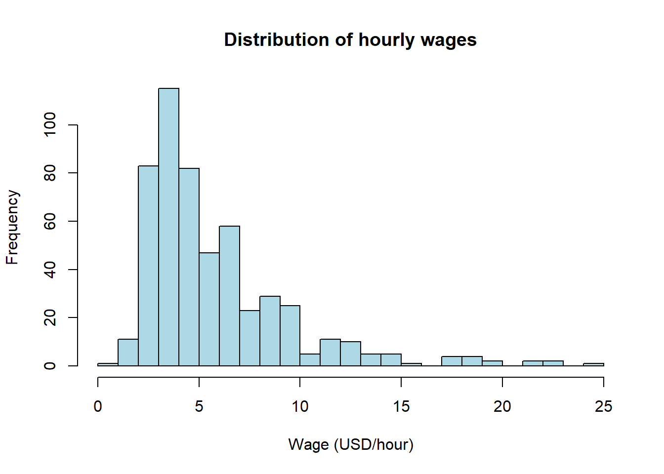
Code
hist(wage1$educ,
     main = "Distribution of years of education",
     xlab = "Years of education",
     col  = "lightgreen",
     breaks = 15)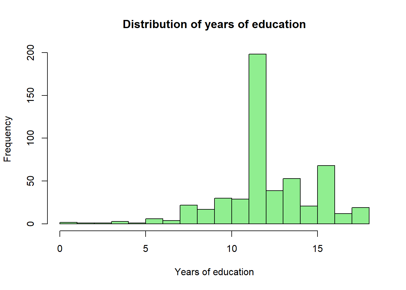
A scatterplot reveals bivariate structure:
Code
plot(wage1$educ, wage1$wage,
     xlab = "Years of education",
     ylab = "Hourly wage (USD)",
     main = "Wage vs. education",
     pch  = 16,
     col  = rgb(0, 0, 1, 0.3))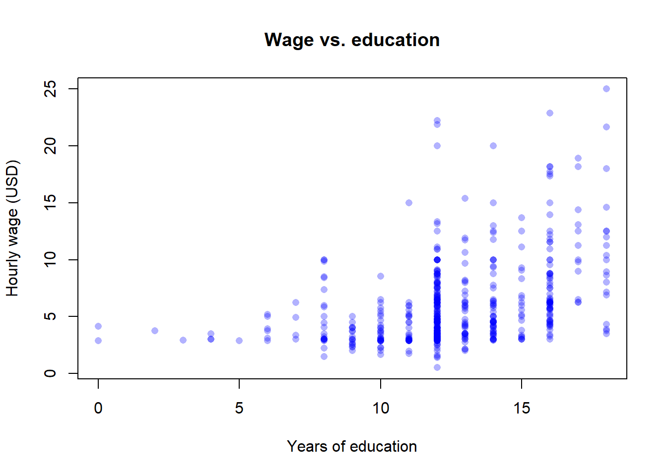
Conditional means — the average of one variable within bins of another — are a non-parametric preview of regression. In base R, tapply() does the job:
Code
tapply(wage1$wage, wage1$educ, mean) 0 2 3 4 5 6 7 8
3.530000 3.750000 2.920000 3.170000 2.900000 3.985000 4.387500 5.038182
9 10 11 12 13 14 15 16
3.275882 3.835667 4.185517 5.371364 5.598974 6.231698 6.321429 8.041618
17 18
11.343333 10.678947 Code
tapply(wage1$wage, wage1$female, mean) 0 1
7.099489 4.587659 The first table is the average wage at each level of education; the second is the average wage by gender. Chapter 1 discusses the interpretation of these numbers at length (and why they are not causal effects). The mechanics of computing them belong here, in the prerequisites.
NoteWhere to go next
Readers who feel rusty on any block above should skim a standard reference before tackling Chapter 2: Wooldridge’s own Appendices A–D are an excellent and notation-consistent companion (Wooldridge 2020). Linear algebra at the level of §A.5 is covered in any first-year text; for a quick refresher tailored to econometrics, see Wooldridge’s Appendix D.
Wooldridge, Jeffrey M. 2020. Introductory Econometrics: A Modern Approach. 7th ed. Cengage Learning.